Max pain & PCR ratio

September 27, 2022August 3, 2022 by Rohansharma

Max pain & PCR ratio

Basics of stock market

• Induction
• Bull call spread
• Bull put spread
• Call ration Back spread
• Bear call ladder
• Synthetic long & Arbitrage
• Bear put spread

• Bear call spread
• put ration back spread
• Long straddle
• Short straddle
• Max pain & PCR ratio
• Iron condor

13.1 – My experience with Option Pain theory

The “Options Pain” theory undoubtedly has a place on the never-ending list of controversial market theories. Option Pain, also known as “Max Pain,” has a sizable fan base, in addition, to probably an equal number of detractors. I’ll be open; I’ve participated on both sides. When I first started investing with Option Pain, I was never able to consistently generate income. Over time, though, I discovered ways to improvise on this theory to fit my own risk tolerance, and that produced a respectable outcome. I’ll go over this as well later in the chapter.

Anyway, this is my attempt to explain the Option Pain theory to you and to discuss my likes and dislikes of Max Pain. This chapter can serve as a guide for how to decide which camp you want to be in.

You must be familiar with the idea of “Open Interest” in order to understand Option Pain theory.

So let’s get going.

13.2 – Max Pain Theory

Here is a step-by-step explanation of how to determine the Max Pain value. You might find this a little perplexing at this point, but I still advise reading it. Things will become more clear once we use an example.

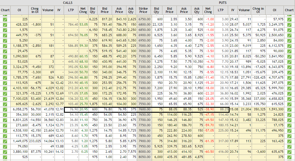
Step 1: Make a list of the different exchange strikes and note the open interest in calls and puts for each strike.

Step 2: Assume that the market will expire at each of the strike prices you have noted.

Step 3: Assuming the market expires as per the assumption in step 2, figure out how much money is lost by option writers (both call option and put option writers).

Step 4: Total the money that calls and put option writers have lost.

Step 5: Determine the strike at which option writers lose the least amount of money.

The point at which option buyers experience the most suffering is the level at which option writers lose the least amount of money. The market will therefore most likely end at this price.

Let’s use a very straightforward example to illustrate this. I’ll assume there are only 3 Nifty strikes available in the market for the purposes of this example. I have noted the open interest for the respective strike for both call and put options.

Situation 1: Assume that the market closes at 7700

Keep in mind that you will only lose money when writing a call option if the market rises above the strike. Similarly, you will only lose money when the market moves below the strike price when you write a put option.

Therefore, none of the call option writers will experience a loss if the market expires at 7700. Therefore, the premiums received by call option writers for the 7700, 7800, and 7900 strikes will be kept.

The writers of put options, however, will have difficulties. The 7900 PE writers will be discussed first.

7900 PE writers would lose 200 points at the 7700 expiries. OI being 2559375, the loss in rupees would be equal to –

= 200 * 2559375 = Rs.5,11,875,000/-

7800 PE writers would suffer a 100 loss.

= 100 * 4864125 = Rs.4,864,125,000/-

It won’t cost 7700 PE writers any money.

Therefore, if the markets expire at 7700, the total amount of money lost by option writers would be –

Call option writers’ total losses plus put option writers’ total losses

= 0 + Rs.511875000 + 4,864125000 = Rs.9,98,287,500/-

Remember that the total amount of money lost by call option writers equals the sum of the losses suffered by writers of 7700 CE, 7800 CE, and 7900 CE.

Similarly, the total amount of money lost by put option writers is equal to the sum of the losses of the writers of the 7700 PE, the 7800 PE, and the 7900 PE.

Scenario 2: Assume that the market closes at 7800.

The writers of the following call options would lose money at 7800:

Using its Open, 7700 CE writers would lose 100 points.

get the loss’s rupee value.

100*1823400 = Rs.1,82,340,000/-

Sellers of the 7800 CE and 7900 CE would both make money.

The seller of the 7700 and 7800 PE wouldn’t suffer a loss.

The loss in rupees would be equal to 100 points for the 7900 PE, multiplied by the open interest.

100*2559375 = Rs.2,55,937,500/-

Therefore, when the market expires at 7800, the total loss for option writers would be –

= 182340000 + 255937500

= Rs.4,38,277,500/-

Scenario 3 – Assume markets expire at 7900

At 7900, the following call option writers would lose money –

7700 CE writer would lose 200 points, the Rupee value of this loss would be –

200 *1823400 = Rs.3,646,800,000/-

7800 CE writer would lose 100 points, and the Rupee value of this loss would be –

100*3448575 = Rs.3,44,857,500/-

7900 CE writers would retain the premiums received.

Since market expires at 7900, all the put option writers would retain the premiums received.

So therefore the combined loss of option writers would be –

= 3646800000 + 344857500 = Rs. 7,095,375,000/-

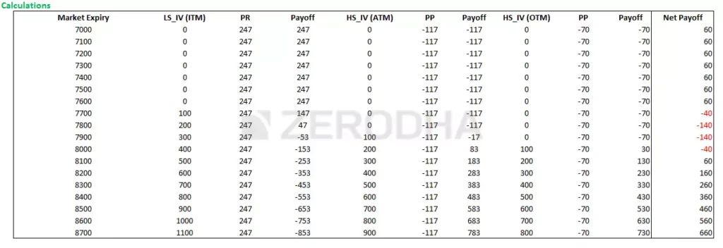
So at this stage, we have calculated the total Rupee value loss for option writers at every possible expiry level. Let me tabulate the same for you –

get the loss’s rupee value.

100*1823400 = Rs.1,82,340,000/-

We can quickly determine the point at which the market is likely to expire now that we have determined the combined loss that option writers would sustain at various expiry levels.

According to the theory of option pain, the market will expire at a point where option sellers will experience the least amount of suffering (or loss).

The combined loss at this point (7800), which is significantly less than the combined loss at 7700 and 7900, is approximately 43.82 Crores, as can be seen from the table above.

That is all there is to the calculation. For the sake of simplicity, I’ve only used 3 strikes in the example.

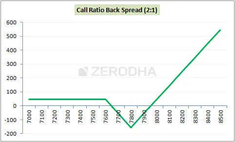
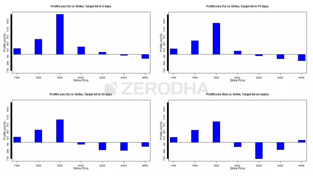
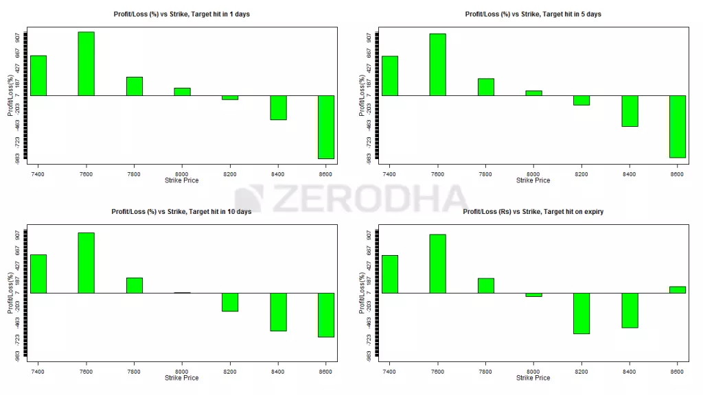
For all the available strikes, we assume the market would expire at that point and then compute the Rupee value of the loss for CE and PE option writers. This value is shown in the last column titled “Total Value”. Once you calculate the total value, you simply have to identify the point at which the least amount of money is lost by the option writer. You can identify this by plotting the ‘bar graph’ of the total value. The bar graph would look like this –

As you can see, the 7800 strike is where option writers would lose the least money, so in accordance with the theory of option pain, this is the strike where the market for the May series is most likely to expire.

How can you put this information to use now that you’ve determined the expiry level? Well, there are many applications for this knowledge.

The majority of traders identify the strikes they can write using this maximum pain level. Since 7800 is the anticipated expiration level in this scenario, one can choose to write call options above 7800 or put options below 7800 and keep all of the premiums.

As a result, I eventually modified the traditional option pain theory to fit my risk tolerance. What I did was as follows:

Every day, the OI values change. As a result, the option pain may suggest 8000 as the expiry level on May 20 and 7800 as the expiry level on May 10. To perform this calculation, I froze on a specific day of the month. When there were 15 days left until expiration, I preferred to do this.

In accordance with the standard option pain method, I determined the expiry value.
I would include a “safety buffer” of 5%. The theory suggests 7800 as the expiry at 15 days, so I would then add a 5 percent safety buffer. As a result, the expiration value would be 7800 plus 5% of 7800.

The market could end anywhere between 7800 and 8200, in my opinion.
I would create strategies with this expiration range in mind, with writing call options beyond 8200 being my favourite.
Simply put,

I wouldn’t write a put option because panic spreads more quickly than greed. This implies that markets may decline before rising.

I would typically refrain from averaging during this time and instead hold the sold options until they expired.

13.5 – The Put Call Ratio

Calculating the Put Call Ratio is a fairly straightforward process. The ratio enables us to determine whether the market is extremely bullish or bearish. The PCR test is typically used as a contrarian indicator. In other words, if the PCR shows extreme bearishness, we expect the market to turn around, so the trader adopts a bullish stance. Likewise, traders anticipate a market reversal and decline if the PCR shows extreme bullishness.

Simply dividing the total open interest of Puts by the total open interest of Calls yields the PCR formula. The outcome typically ranges in and around one. Look at the illustration below:

As of 10^th May, the total OI of both Calls and Puts has been calculated. Dividing the Put OI by Call OI gives us the PCR ratio –

37016925 / 42874200 =

0.863385

The following interpretation is correct:

If the PCR value is higher than 1, say 1.3, it means that more puts than calls are being purchased. This indicates that the markets have become very bearish and are thus somewhat oversold. Search for reversals and anticipate an increase in the markets.

Low PCR values, such as 0.5 and below, show that more calls than puts are being purchased. This indicates that the markets have become very bullish and are thus somewhat overbought. One can watch for reversals and anticipate a decline in the markets.
It is possible to attribute all values between 0.5 and 1 to normal trading activity, so they can all be disregarded.

This is obviously a general approach to PCR. It would be sensible to identify these extreme values by historically plotting the daily PCR values over, say, a period of one or two years. For instance, a value of 1.3 for the Nifty can signify extreme bearishness, whereas 1.2 for the Infy could mean the same thing. You must understand this, so backtesting is helpful.

Why PCR is used as a contrarian indicator may be a mystery to you. The reason for this is a little difficult to understand, but the general consensus is that if traders are bullish or bearish, then the majority of them have already taken their respective positions (hence a high/low PCR), and there aren’t many other players who can enter and move the positions in the desired direction. Therefore, when the position eventually squares off, the stock or index will move in the opposite direction.

That’s PCR for you, then. There are numerous variations of this that you may encounter. Some prefer to take volumes instead of OI, while others prefer to take the total traded value. But I don’t believe that overanalyzing PCR is necessary.

13.6 – Final thoughts

And with that, I’d like to conclude the 36 chapters and two modules long module on options!

In this module, we have covered nearly 15 different option strategies, which, in my opinion, is more than enough for retail traders to engage in profitable options trading. Yes, you will come across many fancy option strategies in the future; perhaps your friend will suggest one and demonstrate its technicalities but keep in mind that fancy does not necessarily equate to profitable. The best tactics can sometimes be straightforward, elegant, and straightforward to use.

The information we’ve provided in Modules 5 and 6 are written with the goal of providing you with a clear understanding of what options trading is.

What can be accomplished with options trading and what cannot? What is necessary and what is not have both been considered and discussed. Since these two modules cover the majority of your questions and concerns about options, they are more than enough.

So kindly read through the information provided here at your own pace, and I’m confident you’ll soon begin trading options the right way.

Last but not least, I sincerely hope you enjoy reading this as much as I did writing it for you.

Good luck and keep making money!

For Visit: Click here to know the Directions.

Short straddle

September 27, 2022August 3, 2022 by Rohansharma

Short straddle

Basics of stock market

• Induction
• Bull call spread
• Bull put spread
• Call ration Back spread
• Bear call ladder
• Synthetic long & Arbitrage
• Bear put spread

• Bear call spread
• put ration back spread
• Long straddle
• Short straddle
• Max pain & PCR ratio
• Iron condor

11.1 – Context

In the previous chapter we understood that for the long straddle to be profitable, we need a set of things to work in our favor, reposting the same for your quick reference –

The volatility should be relatively low at the time of strategy execution
The volatility should increase during the holding period of the strategy
The market should make a large move – the direction of the move does not matter
The expected large move is time bound, should happen quickly – well within the expiry
Long straddles are to be set up around major events, and the outcome of these events is to be drastically different from the general market expectation.

Although it is acknowledged that the long straddle does not depend on the direction of the market, this is a very difficult bargain. Considering the five points listed, it can be difficult to make the long straddle work in your favour. Remember that the breakdown in the previous chapter was at 2%; add another 1% for desired profits, and we are essentially looking for at least a 3% movement on the index. According to my experience, it can be difficult to anticipate the market’s frequent changes. In fact, just for this reason, I pause every single time I need to start a long straddle.

I’ve seen a lot of traders carelessly set up long straddles in the mistaken belief that they are protected from the direction of the market. However, in reality, they lose money in a long straddle because of time delays and the market’s overall movement (or lack thereof). Please note that I’m not trying to convince you not to use the long straddle; nobody contests its simplicity and elegance. When all five of the aforementioned criteria are met, it functions incredibly well. The likelihood of these 5 points aligning with one another is the only problem I have with long straddle.

Consider this: A number of factors prevent the long straddle from being profitable. Therefore, as a continuation of this, the same set of factors “should” favour the “Short Straddle,” which is the opposite of a long straddle.

11.2 – The Short Straddle

Although many traders fear the short straddle (as losses are uncapped), I personally prefer trading the short straddle on certain occasions over its peer strategies. Anyway, let us quickly understand the setup of a short straddle, and how its P&L behaves across various scenarios.

Setting up a short straddle is quite straightforward – as opposed to buying the ATM Call and Put options (like in a long straddle) you just have to sell the ATM Call and Put option. Obviously, the short strategy is set up for a net credit, as when you sell the ATM options, you receive the premium in your account.

Here is an example, consider Nifty is at 7589, so this would make the 7600 strike ATM. The option premiums are as follows –

7600 CE is trading at 77
7600 PE is trading at 88

So the short straddle will require us to sell both these options and collect the net premium of 77 + 88 = 165.

Please keep in mind that the options must have the same underlying, the same expiration date, and of course, the same strike. Let’s calculate the P&L under various market expiry scenarios assuming that you have already executed this short straddle.

Situation 1: The market closes at 7200 (we lose money on the put option)

In this case, the put option’s loss is so sizable that it consumes the premium that both the CE and the PE collected, resulting in a net loss. At 7200 –

As a result of the fact that 7600 CE will expire worthlessly, we keep the premium received, meaning that 77 7600 PE will have an intrinsic value of 400. When the premium received, Rs. 88, is taken into account, we lose 400 – 88 = – 312.
312 – 77 = – 235 would be the overall loss.
As you can see, the loss in the put option equals the gain in the call option.

The market expires at 7435 in scenario two (lower breakdown)

In this instance, the strategy is in a neutral financial position.

Since 7600 CE would expire worthlessly, the premium is kept. Profit is Rs. 77 here.
Since we received Rs. 88 in premium on an intrinsic value of 165 for 7600 PE, our loss would be 165 – 88 = -77.
The loss in the put option completely cancels out the gain in the call option. Consequently, at 7435, we are in the black.

Situation 3: The market closes at 7600 (at the ATM strike, maximum profit)

The best result for a short straddle is this one. The situation is simple at 7600 because both the call and put options would expire worthlessly and the premiums from both the call and put options would be kept. The gain, in this case, would equal the net premium received, or Rs. 165.

This indicates that in a short straddle, you profit the most when the markets remain static.

The market expires at 7765 in scenario 4. (upper breakdown)

This is comparable to the second scenario we looked at. At this point, the strategy achieves parity at a point above the ATM strike.

After accounting for the premium of Rs. 77 that was received, 7600 CE would have an intrinsic value of Rs. 165, meaning that we would lose Rs. 88. (165 – 77)
7600 PE would expire worthlessly, so the premium, which is equal to Rs. 88, is kept.

We are neither making money nor losing money because the profit from the 7600 PE is offset by the loss from the 7600 CE.

This is undoubtedly the upper breakdown point.

In this case, the market is obviously much larger than the 7600 ATM threshold. Both the loss and the call option premium would increase.7600 PE will expire worthlessly, so the premium, which is equal to Rs. 88, is kept.

After accounting for the premium of Rs. 77 received, the 7600 CE will have an intrinsic value of Rs. 400 at 8000, meaning that we will lose Rs. 323. ( 400 -77)
Given that we paid Rs. 88 as the put option premium, our loss would be equal to 88 – 323 = –235.

As you can see, the call option’s loss is sizable enough to cancel out the total premiums paid.

The payoff table for various market expiries is shown below.

11.3 – Case Study (repost from previous module)

He decided to proceed with the 1140 strike because Infosys was trading close to Rs. 1142/- per share (ATM).

Here is the snapshot taken at the time the trade was started:

The 1140 CE was trading at 48/- on October 8 around 10:35 AM, and the implied volatility was 40.26 percent. The implied volatility was 48 percent and the 1140 PE was trading at 47/-. 95 dollars per lot were received in total premium.

The market anticipated that Infosys would release a respectable set of financial results. In fact, the results were better than anticipated; the specifics are as follows:

“Information Systems reported a net profit of $519 million for the July-September quarter, up from $511 million in the same period last year. The amount of revenue increased by 8.7% to $2.39 billion. Revenue increased by 6% sequentially, comfortably exceeding market expectations of growth of 4- 4.5%.

On revenues of Rs. 15,635 crores, which was up 17.2 percent from the previous year, net profit increased by 9.8 percent to Rs. 3398 crores in rupees. Economic Times is the source.

Three minutes after the market opened and around the time of the announcement, at 9:18 AM, this trader was able to close the trade.

5.4 – Effect of Greeks

Since we are dealing with ATM options, the delta of both CE and PE would be around 0.5. We could add the deltas of each option and get a sense of how the overall position deltas behave.

Given that we are short, the delta for the 7600 CE would be -0.5.
Since we are short, the delta for the 7600 PE Delta would be +0.5.
Delta added together would be -0.5 + 0.5 = 0.
The total delta shows that the tactic is neutral in terms of direction. Keep in mind that a delta-neutral straddle can be either long or short. Delta neutral suggests that the profits are uncapped for long straddles and the losses are uncapped for short straddles.

Here’s something to consider: When you start a straddle, you are undoubtedly delta neutral. But will your position still be delta neutral as the markets change? If so, why do you believe that? If the answer is no, is there a way to maintain a neutral position delta?

I can assure you that your understanding of options is far superior to that of 90% of market participants if you can structure your thinking around these ideas. You must take a small mental step forward and enter second-level thinking in order to respond to these straightforward questions.

For Visit: Click here to know the directions.

Long straddle

September 27, 2022August 3, 2022 by Rohansharma

Long straddle

Basics of stock market

• Induction
• Bull call spread
• Bull put spread
• Call ratio Back Spread
• Bear call ladder
• Synthetic long & Arbitrage
• Bear put spread

• Bear call spread
• put ration back spread
• Long straddle
• Short straddle
• Max pain & PCR ratio
• Iron condor

10.1 – The Directional dilemma

How often do you find yourself in a position where you decide to trade long or short after giving it a lot of thought, only to see the market move in the exact opposite direction shortly thereafter? Your entire plan, strategy, work, and resources are wasted. I’m positive that we have all been in a situation like this. In fact, this is one of the main reasons why most experienced traders adopt a variety of directional betting strategies that are resistant to the unpredictability of the market.

Market Neutral or Delta Neutral strategies are those whose profitability is largely independent of market direction. In the upcoming chapters, we’ll learn about some market-neutral tactics and how Such trading tactics can be used by everyday retail traders. Let’s start off with a “Long Straddle.”

10.2 – Long Straddle

The simplest market-neutral strategy to use is probably the long straddle. The direction that the market moves has no bearing on the P&L once it has been implemented. The market must move, regardless of the direction, it moves in. A positive P&L is produced as long as the market is moving (regardless of the direction it is moving). All that is required to execute a long straddle is –

Buy a Call option
Buy a Put option

Ensure –

Both the options belong to the same underlying
Both the options belong to the same expiry
Belong to the same strike

Here is an illustration of how to execute a long straddle and how the overall strategy performed. The market is currently trading at 7579, making the strike price of 7600 “At the money” as of the time of this writing. We would have to buy the ATM call and put options simultaneously if we wanted to long straddle.

Based on the scenarios discussed above, we can draw a few conclusions:

Technically speaking, this is a ladder and not a spread. The first two option legs, however, produce a traditional “spread” in which we sell ITM and buy ATM. It is possible to interpret the spread as the difference between ITM and ITM options. It would be 200 in this instance (7800 – 7600).
Net Credit equals Premium collected from ITM CE minus Premium paid to ATM and OTM CE
Spread (difference between the ITM and ITM options) – Net Credit equals the maximum loss.
When ATM and OTM Strike, Max Loss occurs.
When the market declines, the reward equals Net Credit.
Lower Strike plus Net Credit equals Lower break-even.
Upper Breakeven is equal to the sum of the long strike, short strike, and net premium.

Take note of how the strategy loses money between 7660 and 8040 but ends up profiting greatly if the market rises above 8040. You still make a modest profit even if the market declines. However, if the market does not move at all, you will suffer greatly. Because of the Bear Call Ladder’s characteristics, I advise you to use it only when you are positive that the market will move in some way, regardless of the direction.

In my opinion, when the quarterly results are due, it is best to use stocks (rather than an index) to implement this strategy.

10.3 – Effect of Greeks

Volatility does play a significant role when using the straddle. If I said that volatility makes or breaks the straddle, I wouldn’t be exaggerating. Therefore, the success of the straddle depends on a fair assessment of volatility. View the graph below for more information.

The cost of the strategy is shown on the y-axis, which is just the sum of the option premiums, and volatility is shown on the x-axis. With 30, 15, and 5 days until expiration, the blue, green, and red lines show, respectively, how the premium rises as volatility rises. As you can see, this is a linear graph, and regardless of the time until expiration, the cost of the strategy rises as volatility does. In a similar vein, strategy costs drop as volatility does.

Look at the blue line; it indicates that setting up a long straddle will cost you 160 when volatility is 15%. Keep in mind that the price of a long straddle is equal to the total premium needed to purchase both call and put options. When volatility is 15%, setting up a long straddle costs Rs. 160; however, assuming all other factors remain the same, when volatility is 30%, setting up the same long straddle costs Rs. 340. So long as – you are likely to double your investment in the straddle.

You set up the long straddle at the start of the month
The volatility at the time of setting up the long straddle is relatively low
After you set up the long straddle, the volatility doubles

Similar observations can be drawn from the green and red lines, which show the price to volatility behavior at 15 and 5 days from expiration, respectively. This also means that if you execute the straddle when volatility is high and declines after you execute the long straddle, you will lose money. This is a very important thing to keep in mind. Let’s now quickly talk about the delta of the overall strategy. Since we are long on the ATM strike, both options’ deltas are close to 0.5.

The call option has a delta of + 0.5
The put option has a delta of – 0.5

The delta of the call option cancels out the delta of the put option, leaving a net delta of zero. Remember that delta displays the bias in the position’s direction. A bullish bias is indicated by a +ve delta, whereas a bearish bias is indicated by a -ve delta. Given this, a 0 delta means that there is absolutely no bias toward the market’s direction. Therefore, all strategies with zero deltas are referred to as “Delta Neutral,” and Delta Neutral strategies are protected from the direction of the market.

10.4 – What can go wrong with the straddle?

On the surface, a long straddle appears fantastic. Consider the fact that you stand to gain financially regardless of how the market performs. All you require is an accurate estimation of volatility. So what could possibly go wrong with a straddle? Well, two things stand in the way of your ability to profit from a long straddle.

Theta Decay – In the absence of other factors, options are depreciating assets, which is especially detrimental to long positions. The time value of the option decreases as expiration draws nearer. Holding onto out-of-the-money or in-the-money options into the final week before expiration will result in rapid premium loss because time decay accelerates exponentially during this period.

Remember that the break-even points in the earlier example we discussed were 165 points away from the ATM strike. Taking into account the ATM strike at 7600, the lower breakeven point was 7435 and the upper breakeven point was 7765. To achieve breakeven, the market must move 2.2 percent (either way) in percentage terms. This means that for you to start profiting from the time you start the straddle, the market or the stock must move at least 2.2 percent in either direction. and this transfer must be completed in no more than 30 days. Furthermore, a move of 1 percent over and above 2.2 percent on the index is required if you want to make a profit of at least 1 percent on this trade. A significant change in the index

We can sum up what really needs to go in your favor for the straddle to be profitable by keeping the previous two points plus the effect on volatility in perspective.

When applying the strategy, the volatility ought to be quite low.

During the strategy’s holding period, the volatility should rise.

The market should move significantly; it makes no difference in which way it moves.

The anticipated large move is time-bound and ought to occur quickly – well before the expiration

My trading long straddles have taught me that they are profitable when placed around significant market events, and the impact of such events should be greater than what the market anticipates. Please read the following paragraphs carefully as I will go into more detail about the “event and expectation” part. Consider the Infosys outcomes as an illustration.

Event – Quarterly results of Infosys

Expectation – ‘Muted to flat’ revenue guideline for the coming few quarters.

Actual Results: Infosys announced a “muted to flat” revenue guideline for the upcoming quarters, as was predicted. A long straddle would probably collapse if it were set up against the backdrop of such an event (and its expectation), and eventually, the expectation would be met. This is due to the fact that volatility tends to rise around significant events, which tends to raise premiums.

In other words, if you buy ATM calls and put options close to an event, you are essentially buying options at a time of high volatility. When events are made public and the result is known, the volatility and consequently the premiums fall like a stone. Due to the “bought at high volatility and sold at low volatility” phenomenon, this naturally breaks the straddle down, causing the trader to lose money. I frequently see this happening, and regrettably, I’ve seen plenty of traders lose money precisely because of it.

Favorable Outcome – Now imagine that they announce an “aggressive” guideline in place of the “muted to flat” guideline. This would essentially catch the market off guard and raise premiums significantly, making for a successful straddle trade. This indicates that there is a different perspective to consider: you should evaluate the outcome of the event a little more favorably than the market as a whole.

A straddle cannot be set up with a subpar evaluation of the events and their result. This may seem like a challenging proposition, but trust me when I say that a few good years of trading experience will actually enable you to assess situations far more accurately than the market as a whole. In order to be clear, I’d like to reiterate all the angles that must line up for the straddle to be profitable:

The volatility should be relatively low at the time of strategy execution
The volatility should increase during the holding period of the strategy
The market should make a large move – the direction of the move does not matter
The expected large move is time-bound and should happen quickly – well within the expiry
Long straddles are to be set around major events, and the outcome of these events is to be drastically different from the general market expectation.

For Visit: Click here to know the directions.

Put ration back spread

September 27, 2022August 1, 2022 by Rohansharma

Background of Bear call ladder

Basics of stock market

• Induction
• Bull call spread
• Bull put spread
• Call ration Back spread
• Bear call ladder
• Synthetic long & Arbitrage
• Bear put spread

• Bear call spread
• put ration back spread
• Long straddle
• Short straddle
• Max pain & PCR ratio
• Iron condor

4.1 – Background of Bear call ladder

In this module’s chapter 4, we covered the “Call Ratio Back spread” strategy in great detail. Similar to the Call ratio back spread, the Put ratio back spread is used by traders who are bearish on the market or a particular stock.

This is essentially what will happen when you use the Put Ratio Back Spread.

Unlimited profit if the market goes down
Limited profit if the market goes up
A predefined loss if the market stays within a range

Simply put, you profit whether the market moves up or down. Of course, the strategy is more advantageous if the market declines.

The Put Ratio Back Spread is typically used for a “net credit,” which means that money starts to arrive in your account as soon as you execute the strategy. In contrast to what you anticipate, the “net credit” is what you earn if the market rises (i.e market goes down). On the other hand, if the market does indeed decline, you will profit indefinitely.

This should also clarify why purchasing a plain vanilla put option is preferable to the put ratio back spread.

4.2 – Strategy Notes

As it involves purchasing two OTM Put options and selling one ITM Put option, the Put Ratio Back Spread is a three-legged option strategy. This is the standard 2:1 combination. The put ratio back spread must actually be executed in a 2:1 ratio, which means that two options must be purchased for every one option sold, or three options must be purchased for every two options sold, and so on.

Let’s use the Nifty Spot at 7506 as an example. You predict that Nifty will reach 7000 by expiration. This is unmistakably a pessimistic expectation. The Put Ratio Back Spread should be used if:

Sell one lot of 7500 PE (ITM)
Buy two lots of 7200 PE (OTM)

Make sure –

The Put options belong to the same expiry
Belong to the same underlying
The ratio is maintained

The trade set up looks like this –

7500 PE, one lot short, the premium received for this is Rs.134/-
7200 PE, two lots long, the premium paid is Rs.46/- per lot, so Rs.92/- for 2 lots
Net Cash flow is = Premium Received – Premium Paid i.e 134 – 92 = 42 (Net Credit)

Situation 1: The market closes at 7600 (above the ITM option)

Both Put options would expire worthless at 7600. Following are the intrinsic value of options and the ultimate strategy payoff:

7500 PE would also expire worthless, but we have written this option and received a premium of Rs.134, which in this case can be retained back. 7200 PE would also expire worthless, but since we are long 2 lots of this option at a cost of Rs.46 per lot, we would lose the entire premium of Rs.92 paid.
134 – 92 = 42 is the strategy’s net payoff.
Keep in mind that the strategy’s net payoff at 7600 (higher than the ITM strike) is equal to the net credit.

The market expires in scenario 2 at 7,500. (at the higher strike i.e the ITM option)

Both options would expire worthless at 7500 because neither would have any intrinsic value. As a result, the reward would be comparable to the reward we discussed at 7600. As a result, the net strategy payoff would be Rs. 42. (net credit).

In actuality, as you might have guessed, the strategy’s payoff at any point above 7500 equals the net credit.

The market expires in scenario 2 at 7,500. (at the higher strike i.e the ITM option)

In actuality, as you might have guessed, the strategy’s payoff at any point above 7500 equals the net credit.

The entire premium paid, or $92, will be lost because the 7200 PE has no intrinsic value.
Therefore, we would lose 92 on the 7200 PE while making 92 on the 7500 PE, resulting in no loss and no gain. As a result, one of the breakeven points is 7458.

Scenario 4 – Market expires at 7200 (Point of maximum pain)

This is the point at which the strategy causes maximum pain, let us figure out why.

At 7200, 7500 PE would have an intrinsic value of 300 (7500 – 7200). Since we have sold this option and received a premium of Rs.134, we would lose the entire premium received and more. The payoff on this would be 134 – 300 = – 166
7200 PE would expire worthless as it has no intrinsic value. Hence the entire premium paid of Rs.92 would be lost
The net strategy payoff would be -166 – 92 = – 258
This is a point where both the options would turn against us, hence is considered as the point of maximum pain

5.3 – Strategy Generalization

Based on the scenarios discussed above, we can draw a few conclusions:

Technically speaking, this is a ladder and not a spread. The first two option legs, however, produce a traditional “spread” in which we sell ITM and buy ATM. It is possible to interpret the spread as the difference between ITM and ITM options. It would be 200 in this instance (7800 – 7600).
Net Credit equals Premium collected from ITM CE minus Premium paid to ATM and OTM CE
Spread (difference between the ITM and ITM options) – Net Credit equals the maximum loss.
When ATM and OTM Strike, Max Loss occurs.
When the market declines, the reward equals Net Credit.
Lower Strike plus Net Credit equals Lower Breakeven.
Upper Breakeven is equal to the sum of the long strike, short strike, and net premium.

In my opinion, when the quarterly results are due, it is best to use stocks (rather than an index) to implement this strategy.

5.4 – Effect of Greeks

I assume you are already familiar with these graphs. The following graphs demonstrate the profitability of the strategy taking into account the time until expiration; as a result, these graphs assist the trader in choosing the appropriate strikes.

The best strikes to choose are deep ITM and slightly ITM, i.e., 7600 (lower strike short) and 7900, if you expect the move during the second half of the series and you expect it to happen within a day (or within 5 days, graph 2). (higher strike long). Please take note that this is an ITM and ITM spread rather than the traditional combination of an ITM + OTM spread. In actuality, none of the other combinations work.

Graphs 3 (bottom right) and 4 (bottom left): The best strategy is to use these graphs if you anticipate a move during the second half of the series and that it will occur within 10 days (or on the expiry day, graph 4).Deep ITM and slightly ITM strikes, such as 7600 (lower strike short) and 7900, are the best options (higher strike long). This is in line with what graphs 1 and 2 indicate.

The relationship between the change in “premium value” and the change in volatility is shown by three coloured lines. These lines make it easier for us to comprehend how an increase in volatility affects the strategy while keeping the time until expiration in mind.

Green line – This line suggests that, although not as much as in the preceding case, an increase in volatility is advantageous when there are roughly 15 days until expiration. As we can see, when volatility rises from 15% to 30%, the strategy payoff increases from -77 to -47.

Red line: Clearly, the premium value is not significantly affected by an increase in volatility as time approaches expiration. This indicates that when expiration is approaching, you should only be concerned with directional movement and not much with volatility variation.

For Visit: Click here to know the directions.

Bear call spread

August 1, 2022 by Rohansharma

Bear Call Spread

Basics of stock market

• Induction
• Bull call spread
• Bull put spread
• Call ration Back spread
• Bear call ladder
• Synthetic long & Arbitrage
• Bear put spread

• Bear call spread
• put ration back spread
• Long straddle
• Short straddle
• Max pain & PCR ratio
• Iron condor

8.1 – Choosing Calls over Puts

The Bear Call Spread is a two-legged option strategy that is used when the market outlook is “moderately bearish,” similar to the Bear Put Spread. In terms of payoff structure, the Bear Call Spread is comparable to the Bear Put Spread, but there are some differences in terms of strategy execution and strike choice. The Bear Call spread entails using call options rather than put options to create a spread (as is the case in bear put spread).

At this point, you might be asking yourself why one would choose a bear call spread over a bear put spread when the payouts from both spreads are comparable.

Strategy Notes

To be honest, a lot will depend on how appealing the premiums are. The Bear Call spread is executed for a credit, as opposed to the Bear Put spread, which is executed for a debit. Therefore, if the market is at a point where –

The markets have rallied considerably (therefore CALL premiums have swelled)
The volatility is favorable
Ample time to expiry

Invoking a Bear Call Spread for a net credit instead of a Bear Put Spread for a net debit makes sense if you have a moderately bearish outlook for the future. Personally, I favour strategies that offer net credit over those that offer net debit.

8.2 – Strategy Notes 2.0

The Bear Call Spread is a two leg spread strategy traditionally involving ITM and OTM Call options. However you can create the spread using other strikes as well. Do remember, the higher the difference between the two selected strikes (spread), larger is the profit potential.The Bear Call Spread is a two leg spread strategy traditionally involving ITM and OTM Call options. However you can create the spread using other strikes as well. Do remember, the higher the difference between the two selected strikes (spread), larger is the profit potential.

Using the bear call spread requires:

Buy 1 OTM Call option (leg 1)
Sell 1 ITM Call option (leg 2)

Ensure –

All strikes belong to the same underlying
Belong to the same expiry series
Each leg involves the same number of options

Let us take up example to understand this better –

Date – February 2016

Outlook – Moderately bearish

Nifty Spot – 7222

Bear Call Spread, trade set up –

Pay Rs. 38 as a premium to purchase a 7400 CE; keep in mind that this is an OTM option. This is a debit transaction because money is being taken out of my account.

Selling the 7100 CE will earn you Rs. 136 as premium; keep in mind that this is an ITM option. This is a credit transaction because I receive money.

Since the net cash flow is positive (136 – 38 = +98), my account has a net credit as a result of the difference between the debit and credit.

A bear call spread is also known as a “credit spread” because, generally speaking, there is always a “net credit” in them. The market may move in any direction and expire at any level after we place the trade. In order to understand what would happen to the bear put spread at various levels of expiry, let’s consider a few scenarios.

The market expires in scenario 1 at 7,500. (above the long Call)

Given that we paid a premium of Rs. 38 for 7400 CE, which has an intrinsic value of 100, we would be in the black by the amount of 100 minus 38, or 62.
The intrinsic value of 7100 CE would be 400, and since we sold this option at Ra.136, we would have suffered a loss of 400 – 136 = -264.
A net loss of -264 + 62 = -202 would result.

The market expires at 7400 in scenario two (at the long call)

The 7100 CE would have intrinsic value at 7400 and would therefore expire in the money. The value of the 7400 CE would expire.

7400 CE would expire worthless, hence the entire premium of Rs.38 would be written of as a loss.
7100 CE would have an intrinsic value of 300, since we have sold this option at Ra.136, we would incur a loss of 300 – 136 = -164
Net loss would be -164 -38 = – 202

Be aware that the loss at 7400 and 7500 are comparable, indicating that the loss is capped at 202 above that point.

The market expires in scenario 3 at 7198. (breakeven)

7198 is regarded as a breakeven point because at this price, the trade is neither profitable nor unprofitable. Let’s look at how these numbers turn out.

The 7100CE would terminate at 7198 with an intrinsic value of 98. Since we sold the option for Rs. 136, we get to keep a portion of the premium, or 136 – 98 = +38. 7400 CE would expire worthless, so we would forfeit the premium, or 38.
This demonstrates unequivocally that at 7198, the strategy is neutrally profitable.

Situation 4: The market closes at 7100 (at the short call)

Both of the Call options would expire worthless at 7100, making them both worthless and out of the money.

7100 will also have no intrinsic value, so the entire premium received, or Rs. 136, will be retained back. 7400 will have no value, so the premium paid will be a complete loss, or Rs. 38.
136 – 38 = 98 would be the net profit.

It is obvious that the strategy generates a profit as and when the market declines.

8.3 – Strategy Generalization

We can generalise the strategy’s key trigger points based on the aforementioned payoff:

Spread: 7400 minus 7100, or the difference between the strikes, is 300.
Net Credit is calculated as Premiums Paid – Premiums Received (136 – 38 = 98).
Lower strike plus Net Credit 7100 + 98 = 7198 to reach breakeven.
Net Credit = Maximum Profit
Maximum Loss: Spread – Net Credit (300 – 98) = 202

At this point, we can sum the Deltas to determine the overall position delta and determine how sensitive the strategy is to directional movement.

I obtained the following Delta values from the BS calculator:

7400 CE has a delta of +0.32 and is an OTM option.
Since we are short 7100 CE, the delta is -(+0.89) = -0.89 since 7100 CE is an ITM option with a delta of +0.89.
Position delta overall is = +0.32 + (-0.89) = -0.57.
The strategy’s negative delta means that it makes money when the underlying value decreases and loses money when the value increases.

8.4 – Strike Selection and impact of Volatility

The graph above explains how the premium varies with respect to variation in volatility and time.

The blue line suggests that the cost of the strategy does not vary much with the increase in volatility when there is ample time to expiry (30 days)
The green line suggests that the cost of the strategy varies moderately with the increase in volatility when there is about 15 days to expiry
The red line suggests that the cost of the strategy varies significantly with the increase in volatility when there is about 5 days to expiry

It is obvious from these graphs that when there is enough time before expiration, one shouldn’t be overly concerned about changes in volatility. However, between the series’ midpoint and its expiration, one should have an opinion on volatility. The bear call spread is best avoided if you anticipate a decrease in volatility; otherwise, it is advised to use it only when an increase is anticipated.

Bear put spread

September 29, 2022July 27, 2022 by Rohansharma

Bear put spread

Basics of stock market

• Induction
• Bull call spread
• Bull put spread
• Call ratio Back Spread
• Bear call ladder
• Synthetic long & Arbitrage
• Bear put spread

• Bear call spread
• put ration back spread
• Long straddle
• Short straddle
• Max pain & PCR ratio
• Iron condor

7.1 – Spreads versus naked positions

Over the last five chapters, we’ve discussed various multi-leg bullish strategies. These strategies ranged to suit an assortment of market outlooks – from an outrightly bullish market outlook to a moderately bullish market outlook.

Reading through the last 5 chapters you must have realized that most professional options traders prefer initiating a spread strategy versus taking on naked option positions. No doubt spreads tend to shrink the overall profitability, but at the same time spreads give you greater visibility on risk. Professional traders value ‘risk visibility’ more than profits. In simple words, it’s a much better deal to take on smaller profits as long as you know what would be your maximum loss under worst-case scenarios.

Spreads have another intriguing feature in that there is always some form of financing involved, with the sale of one option funding the purchase of another. In actuality, one of the primary characteristics that set a spread apart from a typical naked directional position is financing. The strategies you can use when your outlook is neutral to strongly negative will be covered in the following chapters. These strategies share characteristics with the bullish strategies that we covered earlier in the module.

The Bear Put Spread, which is, as you might have guessed, the inverse of the Bull Call Spread, is the first bearish strategy we’ll examine.

4.2 – Strategy Notes

The Bear Put Spread is similarly simple to use as the Bull Call Spread. When the market outlook is moderately bearish,

that is, when you anticipate that the market will decline in the short term but not significantly, you would use a bear put spread. A correction of 4-5 percent would be appropriate if I were to quantify what “moderately bearish” means.

If the markets are correct as anticipated (go down), one would make a modest profit by using a bear put spread; however,

if the markets go up, the trader would only suffer a small loss.

A conservative trader (read as a risk-averse trader) would implement the Bear Put Spread strategy by simultaneously –

Buying an In the money Put option
Selling an Out of the Money Put option

The creation of an ITM and OTM option for the Bear Put Spread is not required. Any two put options can be used to create the bear put spread. The trade’s level of aggression affects the strike decision. But keep in mind that both options must have the same expiration date and underlying. Let’s look at an example and various scenarios to see how the strategy operates in order to better understand the implementation.

Nifty is currently trading at 7485, which means that 7600 PE is in the black and 7400 PE is out of the money.

To use the “Bear Put Spread,” one would have to sell the 7400 PE, and the premium they would receive from doing so would help to pay for the 7600 PE.

In relation to the 7600 PE, the premium received (PR) is Rs. 73, and the premium paid (PP) is Rs. 165.

This transaction’s net debit would be –

We need to take into account various scenarios in order to comprehend how the strategy’s payoff functions under various expiry conditions. Please keep in mind that the payoff occurs at expiration, which means that the trader must hold these positions until expiration.

Situation 1: The market closes at 7800 (above long put option i.e 7600)

In this instance, the market has increased despite expectations that it would decline. Both of the put options at 7800, 7600, and 7400, would have no intrinsic value and would therefore expire worthlessly.

We would keep nothing because the premium we paid for 7600 PE, which was Rs. 165, would become 0.
The premium for the 7400 PE, or Rs. 73, would be kept in full.
Therefore, at 7800, we would experience a loss of Rs. 165 on the one hand, but this would be partially offset by the premium received, which is Rs. 73.
-165 + 73 = -92 would be the total loss.

Please take note that the ‘-ve’ sign next to 165 denotes a money outflow from the account, while the ‘+ve’ sign next to 73 denotes a money inflow into the account.

Additionally, the strategy’s net debit is equal to the strategy’s net loss of 92.

Scenario 2 – Market expired at 7600 (at long put option)

Here, we’ll assume that the market expires at 7600, the price at which we bought the Put option.

Then, at 7600, both the PE for 7600 and the PE for 7400 would expire worthless (similar to scenario 1),

resulting in a loss of -92.

Scenario 3 – Market expires at 7508 (breakeven)

7508 is halfway through 7600 and 7400, and as you may have guessed I’ve picked 7508 specifically to showcase that the strategy neither makes money nor loses any money at this specific point.

The 7600 PE would have an intrinsic value equivalent to Max [7600 -7508, 0], which is 92.
Since we have paid Rs.165 as a premium for the 7600 PE, some of the premium paid would be recovered. That would be 165 – 92 = 73, which means to say the net loss on 7600 PE at this stage would be Rs.73 and not Rs.165
The 7400 PE would expire worthlessly, hence we get to retain the entire premium of Rs.73
So on hand, we make 73 (7400 PE) and on the other, we lose 73 (7600 PE) resulting in a no loss no profit situation

Hence, 7508 would be the breakeven point for this strategy.

Scenario 4 – Market expires at 7400 (at short put option)

This is an interesting level, do recall when we initiated the position the spot was at 7485, and now the market has gone down as expected. At this point, both options would have interesting outcomes.

The 7600 PE would have an intrinsic value equivalent to Max [7600 -7400, 0], which is 200
We have paid a premium of Rs.165, which would be recovered from the intrinsic value of Rs.200, hence after compensating for the premium paid one would retain Rs.35/-
The 7400 PE would expire worthlessly, hence the entire premium of Rs.73 would be retained
The net profit at this level would be 35+73 = 108

The net payoff from the strategy is in line with the overall expectation from the strategy i.e the trader gets to make a modest profit when the market goes down.

Situation 5: The market closes at 7200 (below the short put option)

Again, this is an intriguing level because both possibilities would be valuable in and of themselves.

Let’s determine whether the numbers add up.

The intrinsic value of the 7600 PE would be equal to Max [7600 -7200, 0], which is 400.
After paying back the premium of Rs. 165 that we paid, which would be recovered from the intrinsic value of Rs. 400,

one would still be left with Rs. 235.
The intrinsic value of the 7400 PE would be Max [7400 -7200, 0], which is 200.
We were given a premium of Rs. 73, but we will have to forfeit it and take a loss in excess of Rs. This equals 200 – 73.

7.3 – Strategy critical levels

From the scenarios discussed above, we can generalize the following:

If the spot moves above the breakeven point, the strategy loses money, and if it moves below the breakeven point,

it makes money.
The profits and losses are both limited.
The spread is the variation in the two strike prices.
Spread in this case would be 7600 – 7400 = 200.
Net Debit = Premium Paid – Premium Received, which is 165 – 73, to equal 92.
Higher strike – Net Debit 7600 – 92 = 7508 is the breakeven point.
Max profit is equal to Spread – Net Debit (200 – 92) (108).
Maximum Loss = 92 Net Debit

All of these crucial details can be seen in the strategy payoff diagram:

7.4 – Quick note on Delta

It’s better late than never: I should have included this in the earlier chapters. Every time you use an options strategy, add up the deltas. I calculated the deltas using the B&S calculator.

7600 PE’s delta is -0.618.

-(-0.342)

+ 0.342

Now, since deltas are additive in nature we can add up the deltas to give the combined delta of the position. In this case,

it would be –

-0.618 + (+0.342)

= – 0.276

The ‘-ve’ denotes that the premiums will increase if the markets decline, giving the strategy an overall delta of 0.276.

Similar to the Bull Call Spread, Call Ratio Back spread, and other strategies we’ve discussed in the past, you can add up their deltas and see that they all have a positive delta, indicating that the strategy is bullish.

It becomes very challenging to determine the overall bias of the strategy—whether it is bullish or bearish—when there are more than two option legs. In these situations, you can quickly add up the deltas to determine the bias. Additionally, if the sum of the deltas to zero, the strategy is not particularly biased in any direction.

7.5 – Strike selection and effect of volatility

The strike selection for a bear put spread is very similar to the strike selection methodology of a bull call spread.

0 I hope you are familiar with the ‘1^st half of the series’ and ‘the 2^nd half of the series methodology. If not I’d suggest you kindly read through section 2.3.

Have a look at the graph below –

Choose the following strikes to create the spread if we are in the first half of the series (ample time before expiry) and anticipate a market decline of about 4% from current levels:

The premium varies according to changes in volatility and time, as shown in the graph above.

The blue line indicates that when there is enough time before expiration, the cost of the strategy does not change significantly with the rise in volatility (30 days)
When there are roughly 15 days until expiration, the green line indicates that the cost of the strategy varies moderately

with the rise in volatility.
The red line indicates that with approximately 5 days until expiration, the cost of the strategy varies significantly with the rise in volatility.
These graphs make it obvious that when there is enough time before expiration, one shouldn’t worry too much about changes in volatility. However, one must possess a view of the volatility between the series’ midpoint and its expiration. Only use the bear put spread if you anticipate an increase in volatility; otherwise, avoid using the strategy if you anticipate a decrease in volatility.

4.3 – Strategy Generalization

Going by the above-discussed scenarios we can make a few generalizations –

Spread = Higher Strike – Lower Strike
Net Credit = Premium Received for lower strike – 2*Premium of higher strike
Max Loss = Spread – Net Credit
Max Loss occurs at = Higher Strike
The payoff when the market goes down = Net Credit
Lower Breakeven = Lower Strike + Net Credit
Upper Breakeven = Higher Strike + Max Loss

Here is a graph that highlights all these important points –

4.4 – Welcome back the Greeks

Before understanding the graphs above, note the following –

The nifty spot is assumed to be at 8000
The start of the series is defined as any time during the first 15 days of the series
The end of the series is defined as any time during the last 15 days of the series
The Call Ratio Back Spread is optimized and the spread is created with 300 points difference

The market is predicted to increase by about 6.25 percent, or from 8000 to 8500. In light of the move and the remaining time, the graphs above indicate that –

Top left on Graph 1 and top right on Graph 2 – The most profitable strategy is a call ratio spread using 7800 CE (ITM) and 8100 CE (OTM), where you would sell 7800 CE and buy 2 8100 CE. This is because you are at the beginning of the expiry series and you anticipate the move over the next 5 days (and 15 days in the case of Graph 2) Do keep in mind that even though you would be correct about the movement’s direction, choosing other far OTM strikes call options usually results in losses.

Graphs 3 and 4 (bottom left and bottom right, respectively) – A Call Ratio Spread using 7800 CE (ITM) and 8100 CE (OTM) is the most profitable option if you are at the beginning of the expiry series and anticipate the move in 25 days (and expiry day in the case of Graph 3). In this scenario, you would sell 7800 CE and buy 2 8100 CE.
You must be wondering why the number of strikes is the same regardless of the time remaining. In fact, this is the key: the call ratio back spread functions best when you sell slightly ITM options and buy slightly OTM options with plenty of time left before expiration. In actuality, all other combinations are in the red, particularly those that include far OTM options.

In actuality, none of the other combinations work.

Graphs 3 (bottom right) and 4 (bottom left): The best strategy is to use these graphs if you anticipate a move during the second half of the series and that it will occur within 10 days (or on the expiry day, graph 4). Deep ITM and slightly ITM strikes, such as 7600 (lower strike short) and 7900, are the best options (higher strike long). This is in line with what graphs 1 and 2 indicate.

Three colored lines show the relationship between the change in “net premium,” or the strategy payoff, and the change in volatility. These lines give us insight into how an increase in volatility affects the strategy while keeping the time until expiration in perspective.

The blue line indicates that a rise in volatility with plenty of time left before expiration (30 days) is advantageous for the

call ratio back spread. As we can see, when volatility rises from 15% to 30%, the strategy’s payoff increases from -67 to +43. This obviously implies that when there is enough time before expiration, in addition to being accurate about the direction of the stock or index, you also need to have a view of volatility. Because of this, even though I believe the stock will rise, I would be a little hesitant to use this strategy at the beginning of the series if volatility is higher than average (say more than double the usual volatility reading)

Green line – This line suggests that, although not as much as in the preceding case, an increase in volatility is advantageous when there are roughly 15 days until expiration. As we can see, when volatility rises from 15% to 30%, the strategy payoff increases from -77 to -47.

Red line: This result is intriguing and illogical. The strategy is negatively impacted by an increase in volatility when there are only a few days left until expiration! Consider that a rise in volatility near the expiration date increases the likelihood that the option will expire in the money, which lowers the premium. So, if you are bullish on a stock or index with a few days left until expiration and you anticipate that volatility will rise during this time, proceed with caution.

For Visit: Click here to know the directions.

Synthetic long & Arbitrage

September 27, 2022July 27, 2022 by Rohansharma

Synthetic long & Arbitrage

Basics of stock market

• Induction
• Bull call spread
• Bull put spread
• Call ration Back spread
• Bear call ladder
• Synthetic long & Arbitrage
• Bear put spread

• Bear call spread
• put ration back spread
• Long straddle
• Short straddle
• Max pain & PCR ratio
• Iron condor

6.1 – Background

Imagine being forced to open up long and short positions on Nifty Futures that expire in the same series at the same time. How, and more importantly, why, would you go about doing this?

Both of these issues will be covered in this chapter. Let’s first examine how this can be accomplished, then move on to consider why someone might want to do this (if you are curious, arbitrage is the obvious answer).

Options, as you may already be aware, are extremely flexible derivative instruments that can be used to create any type of payoff structure, including the payoff structure for futures (both long and short futures payoff).

As you can see, the long futures position started at 2360, and since you can’t make money or lose it at that point, it turns the starting point of the position into the breakeven point. If the futures move higher than the breakeven point, you are in the black, and if they move lower than the breakeven point, you are in the red. The amount of profit you make on a move of 10 points upward is exactly equal to the amount of loss you would experience on a move of 10 points downward. The future is also referred to as a linear instrument due to this linearity in the payoff.

The goal of a Synthetic Long is to use options to create a long future payoff that is similar.

4.2 – Strategy Notes

It’s fairly easy to carry out a Synthetic Long; all one needs to do is –

Invest in the ATM Call Option
Vendor Sell ATM Put Option
When you do this, you must ensure that:

The options share the same underlying asset.
has the same expiration
To better understand this, let’s use an illustration. Assuming the Nifty is at 7389, the ATM strike would be 7400. Synthetic Long would require us to short the 7400 PE at 80 and go long on the 7400 CE, which carries a 107-rupee premium.

The difference between the two premiums, or 107 – 80 = 27, would be the net cash outflow.

Consider the following market expiry scenarios:

Situation 1: The market closes at 7200 (below ATM)

Intrinsic value of Put Option = Max [Strike-Spot, 0]

= Max [7400 – 7200, 0]

=Max [200, 0]

= 200.

Clearly, since we are short on this option, we would lose money from the premium we have received. The loss would be –

80 – 200 = -120

The total payoff from the Long Call and Short Put position would be –

= -107 – 120

= -227

Scenario 2 – Market expires at 7400 (At ATM)

Both options would expire worthless if the market closes at precisely 7400.

We forfeit the 107 premium that was paid for the 7400 CE option.

We keep the premium for the 7400 PE option, which is 80.

The combined positions’ net payoff would be -27e 80 – 107.

Keep in mind that 27 is also the strategy’s net cash outflow and the difference between the two premiums.

Scenario 3 – Market expires at 7427 (ATM + Difference between the two premiums)

7427 is an interesting level, this is the breakeven point for the strategy, where we neither make money nor lose money.

7400 CE – the option is ITM and has an intrinsic value of 27. However, we have paid 107 as premium hence we experience a total loss of 80
7400 PE – the option would expire OTM, hence we get to retain the entire premium of 80.
On one hand, we make 80 and on the other, we lose 80. Hence we neither make nor lose any money, making 7427 the breakeven point for this strategy.

6.3 – The Fish market Arbitrage

Both of the call options, 7600 and 7800, would have zero intrinsic value and would therefore expire worthless.

The premium, which amounts to Rs. 201 for the 7600 CE, is ours to keep; however, we forfeit Rs. 156 for the 7800 CE, leaving us with a net reward of Rs. 45.

Situation 3: The market closes at 7645 (at the lower strike price plus net credit)

If you’re wondering why I chose the level of 7645, it’s because this is where the strategy break even is.

7600 CE’s intrinsic value would be:

Spot – Strike Max [0]

= [7645 – 7600, 0]

= 45

Since we sold this option for 201, the option’s net profit would be

201 – 45

On the other hand, we spent an additional 156 to purchase two 7800 CE. We lose the entire premium because it is obvious that the 7800 CE will expire worthless.

The net payoff is:

156 – 156

= 0

6.3 – The Fish market Arbitrage

I’ll assume you have a fundamental knowledge of arbitrage. Arbitrage is the practice of purchasing assets or goods at a discount and then reselling them at a higher price in order to profit from the price difference. Arbitrage trades are almost risk-free when properly executed. I’ll try to give you a straightforward illustration of an arbitrage opportunity.

Assume you reside near a coastal city where fresh sea fish is in plentiful supply; as a result, the price of fish is very low in your city, let’s say Rs. 100 per kg. The same fresh sea fish is in high demand in the nearby city, which is 125 kilometers away. However, the same fish costs Rs. 150 per kg in this neighboring city.

Given this, if you can buy fish in your city for Rs. 100 and sell it in the neighboring city for Rs. 150, you will undoubtedly pocket the difference in price or Rs. 50. Perhaps you’ll need to factor in logistics and transportation costs and only get to keep Rs. 30 per kilogram instead of Rs. 50. This is still a fantastic deal, and this is a typical fish market arbitrage!

If you can buy fish from your city for Rs. 100 and sell it in the neighboring city for Rs. 150, deducting Rs. 20 for expenses, then Rs. 30 per KG is a guaranteed profit with no risk.

If nothing changes, there are no risks involved. However, if circumstances change, your profitability will as well. Here are some potential changes:

No Fish (opportunity risk) – Let’s say you go to the market one day to buy fish for Rs. 100 but there isn’t any to be found. Then you have no chance of earning Rs. 30.
No Buyers (liquidity risk) – You purchase a fish for Rs. 100 and travel to a nearby town to sell it for Rs. 150 when you discover there are no buyers. You are left with nothing more than a bag of dead fish.
Negative bargaining (risk of execution) The fact that you can “always” bargain to buy at Rs. 100 and sell at Rs. 150 is the basis for the entire arbitrage opportunity. What if you happen to buy at 110 and sell at 140 on a bad day? You must still pay 20 forThe arbitrage opportunity would become less appealing, and you might decide not to do this at all if this continued. transport, this means that instead of the usual 30 Rupee profit you get to make only 10 Rupees.

No Fish (opportunity risk) – Assume one day you go to the market to buy fish at Rs.100, and you realize there is no fish in the market. Then you have no opportunity to make Rs.30/-.
No Buyers (liquidity risk) – You buy the fish at Rs.100 and go to the neighboring town to sell the same at Rs.150, but you realize that there are no buyers. You are left holding a bag full of dead fish, literally worthless!
Bad bargaining (execution risk) – The entire arbitrage opportunity hinges upon the fact that you can ‘always’ bargain to buy at Rs.100 and sell at Rs.150. What if on a bad day you happen to buy at 110 and sell at 140? You still have to pay 20 for transport, this means instead of the regular 30 Rupees profit you get to make only 10 Rupees, and if this continues, then the arbitrage opportunity would become less attractive and you may not want to do this at all.
1. Transport becomes expensive (cost of transaction) – This is another crucial factor for the profitability of the arbitrage trade. Imagine if the cost of transportation increases from Rs.20 to Rs.30. Clearly, the arbitrage opportunity starts looking less attractive as the cost of execution goes higher and higher. The cost of the transaction is a critical factor that makes or breaks an arbitrage opportunity
2. Competition kicks in (who can drop lower?) – Given that the world is inherently competitive you are likely to attract some competition who would also like to make that risk-free Rs.30. Now imagine this –
  1. So far you are the only one doing this trade i.e buy fish at Rs.100 and sell at Rs.150
  2. Your friend notices you are making a risk-free profit, and he now wants to copy you. You can’t really prevent this as this is a free market.
  3. Both of you buy at Rs.100, transport it at Rs.20, and attempt to sell it in the neighboring town
  4. A potential buyer walks in and sees there is a new seller, selling the same quality of fish. Who between the two of you is likely to sell the fish to the buyer?
  5. Clearly given the fish is of the same quality the buyer will buy it from the one selling the fish at a cheaper rate. Assume you want to acquire the client, and therefore drop the price to Rs.145/-
  6. The next day your friend also drops the price and offers to sell fish at Rs.140 per KG, therefore igniting a price war. In the whole process, the price keeps dropping and the arbitrage opportunity just evaporates.
  7. How low can the price drop? Obviously, it can drop to Rs.120 (cost of buying fish plus transport). Beyond 120, it does not makes sense to run the business
  8. Eventually, in a perfectly competitive world, competition kicks in and arbitrage opportunity just ceases to exist. In this case, the cost of fish in neighboring towns would drop to Rs.120 or a price point in that vicinity.
I hope the above discussion gave you a quick overview of arbitrage. In fact, we can define any arbitrage opportunity in terms of a simple mathematical expression, for example with respect to the fish example, here is the mathematical equation –

The cost of purchasing fish in town A minus the price of selling fish in town B equals 20.

We essentially have an arbitrage opportunity if there is an imbalance in the equation above. There are arbitrage opportunities in all kinds of markets, including the fish market, the agricultural market, the currency market, and the stock market, and they are all governed by straightforward mathematical equations.

6.4 – The Options arbitrage

There are arbitrage opportunities in almost every market, but to find them and profit from them, one must be a keen observer of the market. Typically, stock market-based arbitrage opportunities let you carry a profit regardless of the market’s direction while locking in a small but guaranteed profit. Due to this, risk-averse traders tend to favor arbitrage trades quite a bit.

Here, I’d like to talk about a straightforward arbitrage scenario that has its roots in the idea of “Put-Call Parity.” Instead of going over the Put-Call Parity theory, I’ll quickly describe one of its applications.

However, to better understand the Put Call Parity, I highly recommend watching this stunning video from Khan Academy.

Interesting, huh? But you might wonder, what’s the catch?

Fees for transactions!

To determine if it still makes sense to execute this trade, one must take into account the execution costs. Think about this:

Brokerage fees, which are assessed on a percentage basis when using a traditional broker, will take a bite out of your gains. As a result, while you initially make 10 points, you might also end up paying 8 to 10 points in brokerage. Your breakeven point on this trade, however, would be roughly 4-5 points if you were to execute it with a discount broker like Zerodha. You now have even more justification to sign up for a Zerodha account.
STT: Keep in mind that the P&L is realized. as a result, you would have to hold your positions until expiration. If you are long an ITM option, which you will be, you will have to pay a sizable STT at expiration. This will further reduce your profits. Please read on to learn more.
Additional taxes that may apply include service tax, stamp duty, and others.
Therefore, it might not be worthwhile to carry an arbitrage trade for 10 points given these expenses. But it would undoubtedly do so if the reward was higher—say, 15 or 20 points. By squaring off the positions just before expiration with 15 or 20 points, you can even escape the STT trap, though it will take a little time.

For Visit: Click here to know the directions.

Bear call ladder

September 29, 2022July 27, 2022 by Rohansharma

Background of Bear Call ladder

Basics of stock market

• Induction
• Bull call spread
• Bull put spread
• Call ratio Back Spread
• Bear call ladder
• Synthetic long & Arbitrage
• Bear put spread

• Bear call spread
• put ratio back spread
• Long straddle
• Short straddle
• Max pain & PCR ratio
• Iron condor

4.1 – Background of Bear Call ladder

You shouldn’t be misled into thinking that the “Bear” in “Bear Call Ladder” refers to a bearish strategy. Since the Bear Call Ladder is a variation on the Call ratio back spread, you should use it only if you are unabashedly bullish on the stock or index.

In fact, In a Bear Call Ladder, selling an “in the money” call option covers the cost of buying call options. Additionally, the Bear Call Ladder is typically configured for a “net credit,” where the cash flow is always superior to the cash flow of the call ratio back spread. But keep in mind that while both of these strategies exhibit comparable payoff structures, their risk structures differ just a little.

4.2 – Strategy Notes

The Bear Call Ladder is a 3 leg option strategy, usually setup for a “net credit”, and it involves –

Selling 1 ITM call option
Buying 1 ATM call option
Buying 1 OTM call

This setup, which uses a 1:1:1 ratio, is known as the Bear Call Ladder. The bear Call Ladder must be executed in a ratio of 1:1:1, meaning that for each ITM Call Option sold, an ATM Call Option and an OTM Call Option must be purchased. Other combinations, such as 2:2:2 or 3:3:3, are possible.

Let’s use an example where the Nifty Spot is at 7790 and you predict it will reach 8100 by expiration. This is unmistakably a market bullish outlook. To put the Bear Call Ladder into practice:

Sell 1 ITM Call option
Buy 1 ATM Call option
Buy 1 OTM Call option

Ensure that
The Call options have the same expiration date.
has the same underlying foundation.
The ratio stays the same.

The trade setup is as follows:

The premium received for this 7600 CE, one lot short, is Rs. 247.
The premium for this option is Rs. 117 for 7800 CE, one lot long.
The premium for this option is Rs. 70/- for 7900 CE, one lot long.
247 – 117 – 70 = 60 would be the net credit.

The bear call ladder is executed using these trades. Let’s examine what would happen to the strategies’ overall cash flow at various levels of expiry.

Please keep in mind that because the strategy payoff is quite flexible, we need to assess it at different levels of expiry.

Scenario 1 – Market expires at 7600 (below the lower strike price)

We know the intrinsic value of a call option (upon expiry) is –

Max [Spot – Strike, 0]

The 7600 would have an intrinsic value of

Max [7600 – 7600, 0]

= 0

Due to the fact that we sold this option, we are able to keep the premium received, which is Rs. 247.

The intrinsic value of the 7800 CE and 7900 CE would both be zero, so we would forfeit the premium payments of Rs. 117 and Rs. 70, respectively, that were made.

Net cash flow would be superior. Paid a premium and received

= 247 – 117 – 70

= 60

The market expires at 7660 in Scenario 2 (lower strike plus received net premium).

The 7600 CE would be worth – on an intrinsic level.

Spot – Strike Max [0]

The 7600’s intrinsic worth would be

Max [7660 – 7600, 0]

= 60

We will subtract 60 from 247 due to the 7600 CE’s shortness, keeping the balance.

= 247 – 60

= 187

The value of the 7800 and 7900 CE would expire, so we would forfeit the premiums paid—117 and 70, respectively.

The full strategic benefit would be:

= 187 – 117 – 70

= 0\

The Put Ratio Back Spread is used in these trades. Let’s examine what would happen to the strategies’ overall cash flow at various levels of expiry.

5.3 – Strategy Generalization

Based on the scenarios discussed above, we can draw a few conclusions:

Technically speaking, this is a ladder and not a spread. The first two option legs, however, produce a traditional “spread” in which we sell ITM and buy ATM. It is possible to interpret the spread as the difference between ITM and ITM options. It would be 200 in this instance (7800 – 7600).
Net Credit equals Premium collected from ITM CE minus Premium paid to ATM and OTM CE
Spread (difference between the ITM and ITM options) – Net Credit equals the maximum loss.
When ATM and OTM Strike, Max Loss occurs.
When the market declines, the reward equals Net Credit.
Lower Strike plus Net Credit equals Lower Breakeven.
Upper Breakeven is equal to the sum of the long strike, short strike, and net premium.

In my opinion, when the quarterly results are due, it is best to use stocks (rather than an index) to implement this strategy.

5.4 – Effect of Greeks

Firstly, Greeks have a similar impact on this strategy as they do on Call Ratio Back spread, particularly in terms of volatility. I’ve copied the discussion on volatility from the previous chapter for your convenience.

undoubtedly, Three colored lines show the relationship between the change in “net premium,” or the strategy payoff, and the change in volatility. These lines give us insight into how an increase in volatility affects the strategy while keeping the time until expiration in perspective.

Blue Line: According to this line, the Bear Call Ladder spread benefits from higher volatility when there are still 30 days until expiration. As we can see, when volatility rises from 15% to 30%, the strategy’s payoff increases from -67 to +43. This obviously implies that when there is enough time before expiration, in addition to being accurate about the direction of the stock or index, you also need to have a view of volatility. Due to this, even though I’m optimistic about the stock, I

would be hesitant to use this strategy at the beginning of the series if volatility is higher than average (say more than double of the usual volatility reading)

Green line – This line suggests that, although not as much as in the preceding case, an increase in volatility is advantageous when there are roughly 15 days until expiration. As we can see, when volatility rises from 15% to 30%, the strategy payoff increases from -77 to -47.

Red line: This result is intriguing and illogical. The strategy is negatively impacted by an increase in volatility when there are only a few days left until expiration! Consider the possibility that a rise in volatility when there are few days left before expiration

As a result of the option’s OTM expiration, the premium drops. So, if you are bullish on a stock or index with a few days left until expiration and you anticipate that volatility will rise during this time, proceed with caution.

Clearly, The best strikes to choose are deep ITM and slightly ITM, i.e., 7600 (lower strike short) and 7900, if you expect the move during the second half of the series and you expect it to happen within a day (or within 5 days, graph 2). (higher strike long). Please take note that this is an ITM and ITM spread rather than the traditional combination of an ITM + OTM spread. In actuality, none of the other combinations work.

Please keep in mind that because the strategy payoff is quite flexible, we need to assess it at different levels of expiry.

At last, The blue line indicates that a rise in volatility with plenty of time left before expiration (30 days) is advantageous for the put ratio back spread. As we can see, when volatility rises from 15% to 30%, the strategy payoff increases from -57 to +10. This obviously implies that when there is enough time before expiration, in addition to being accurate about the direction of the stock or index, you also need to have a view of volatility. Because of this, even though I am bearish on the stock, I might be hesitant to use this strategy at the beginning of the series if volatility is higher than average (say more than double the usual volatility reading)

For Visit: Click here for the directions.

Call ratio Back spread

September 27, 2022July 26, 2022 by Rohansharma

Call ratio Back spread

Basics of stock market

• Induction
• Bull call spread
• Bull put spread
• Call ratio Back Spread
• Bear call ladder
• Synthetic long & Arbitrage
• Bear put spread

• Bear call spread
• put ration back spread
• Long straddle
• Short straddle
• Max pain & PCR ratio
• Iron condor

4.1 – Background of call ratio back spread

A fascinating options strategy is the Call Ratio Back Spread. Considering how easy it is to implement and the kind of payoff it offers the trader, I consider this to be interesting. This should undoubtedly be included in your toolbox of tactics. In contrast to bull call spreads and bull put spreads, which are used when one is only mildly bullish on a stock (or index), this strategy is used when one is outright bullish on it.

When using the Call Ratio Back Spread, you will primarily experience the following:

Unlimited profit if the market goes up
Limited profit if market goes down
A predefined loss if the market stay within a range

In simpler words you can get to make money as long as the market moves in either direction.

The Call Ratio Back Spread is typically used for a “net credit,” which means that money starts to arrive in your account as soon as you execute the strategy. In contrast to what you anticipated, the “net credit” is what you earn if the market declines (i.e market going up). On the other hand, if the market does increase, you could stand to gain an endless amount of money. This should also clarify why purchasing a call ratio spread rather than a standard call option is preferable.

So let’s investigate how this operates right away.

4.2 – Strategy Notes

As it involves purchasing two OTM call options and selling one ITM call option, the Call Ratio Back Spread is a three-legged option strategy. This is the standard 2:1 combination. The call ratio back spread must actually be executed in a 2:1 ratio, which means that two options must be purchased for everyone option sold, four must be purchased for every two options sold, and so on.

Let’s use an example where the Nifty Spot is at 7743 and you predict it will reach 8100 by expiration. This is unmistakably a market bullish outlook. In order to use the Call Ratio Back Spread:

Sell one lot of 7600 CE (ITM)
Buy two lots of 7800 CE (OTM)

Make sure –

The Call options belong to the same expiry
Belongs to the same underlying
The ratio is maintained

The trade set up looks like this –

7600 CE, one lot short, the premium received for this is Rs.201/-
7800 CE, two lots long, the premium paid is Rs.78/- per lot, so Rs.156/- for 2 lots
Net Cash flow is = Premium Received – Premium Paid i.e 201 – 156 = 45 (Net Credit)

The call ratio back spread is used in these trades. Let’s examine what would happen to the strategies’ overall cash flow at various levels of expiry.

Please keep in mind that because the strategy payoff is quite flexible, we need to assess it at different levels of expiry.

The market expires in scenario 1 at 7400. (below the lower strike price)

We are aware that a call option’s intrinsic value (upon expiration) is:

Spot – Strike Max [0]

The 7600’s intrinsic worth would be

Max [7400 – 7600, 0]

= 0

Given that we sold this option, we are entitled to keep the premium received, which is Rs. 201.

Since the intrinsic value of the 7800 call option would also be zero, we would forfeit the entire premium, which works out to 78 rupees per lot or 156 rupees for two lots.

Net cash flow would be superior. Paid a premium and received

= 201 – 156

= 45

Scenario 2 – Market expires at 7600 (at the lower strike price)

Both of the call options, 7600 and 7800, would have zero intrinsic value and would therefore expire worthless.

The premium, which amounts to Rs. 201 for the 7600 CE, is ours to keep; however, we forfeit Rs. 156 for the 7800 CE, leaving us with a net reward of Rs. 45.

Situation 3: The market closes at 7645 (at the lower strike price plus net credit)

If you’re wondering why I chose the level of 7645, it’s because this is where the strategy break even is.

7600 CE’s intrinsic value would be:

Spot – Strike Max [0]

= [7645 – 7600, 0]

= 45

Since we sold this option for 201, the option’s net profit would be

201 – 45

On the other hand, we spent an additional 156 to purchase two 7800 CE. We lose the entire premium because it is obvious that the 7800 CE will expire worthless.

The net payoff is:

156 – 156

= 0

Scenario 3 – Market expires at 7700 (half way between the lower and higher strike price)

The 7600 CE would be intrinsically worth 100, while the 7800 would be worthless.

On the 7600 CE, we keep 101 instead of losing 100 from the 201 premium we received, which is 201 – 100 = 101.

The entire Rs. 156 premium on the 7800 CE is lost, so the strategy yields a total payoff of

= 101 – 156

= – 55

Scenario 4 – Market expires at 8100 (higher than the higher strike price, your expected target)

The intrinsic values of the 7600 CE and 7800 CE will be 500 and 300 respectively.

The final result would be:

Premium Paid for 7800 CE – Premium Received for 7600 CE – Intrinsic Value of 7600 CE + (2* Intrinsic Value of 7800 CE)

= 201 – 500 + (2*300) – 156

= 201 – 500 + 600 -156

= 145

Here are some additional levels of expiration and the strategy’s ultimate reward. Keep in mind that as the market rises, so do the profits, but when the market falls, you still make some money, albeit a small amount.

4.3 – Strategy Generalization

Going by the above discussed scenarios we can make few generalizations –

Spread = Higher Strike – Lower Strike
Net Credit = Premium Received for lower strike – 2*Premium of higher strike
Max Loss = Spread – Net Credit
Max Loss occurs at = Higher Strike
The payoff when market goes down = Net Credit
Lower Breakeven = Lower Strike + Net Credit
Upper Breakeven = Higher Strike + Max Loss

Here is a graph that highlights all these important points –

4.4 – Welcome back the Greeks

Before understanding the graphs above, note the following –

Nifty spot is assumed to be at 8000
Start of the series is defined as anytime during the first 15 days of the series
End of the series is defined as anytime during the last 15 days of the series
The Call Ratio Back Spread is optimized and the spread is created with 300 points difference

The market is predicted to increase by about 6.25 percent, or from 8000 to 8500. In light of the move and the remaining time, the graphs above indicate that –

Top left on Graph 1 and top right on Graph 2 – The most profitable strategy is a call ratio spread using 7800 CE (ITM) and 8100 CE (OTM), where you would sell 7800 CE and buy 2 8100 CE. This is because you are at the beginning of the expiry series and you anticipate the move over the next 5 days (and 15 days in the case of Graph 2) Do keep in mind that even though you would be correct about the movement’s direction, choosing other far OTM strikes call options usually results in losses.

Graphs 3 and 4 (bottom left and bottom right, respectively) – A Call Ratio Spread using 7800 CE (ITM) and 8100 CE (OTM) is the most profitable option if you are at the beginning of the expiry series and anticipate the move in 25 days (and expiry day in the case of Graph 3). In this scenario, you would sell 7800 CE and buy 2 8100 CE.
You must be wondering why the number of strikes is the same regardless of the time remaining. In fact, this is the key: the call ratio back spread functions best when you sell slightly ITM options and buy slightly OTM options with plenty of time left before expiration. In actuality, all other combinations are in the red, particularly those that include far OTM options.

Three colored lines show the relationship between the change in “net premium,” or the strategy payoff, and the change in volatility. These lines give us insight into how an increase in volatility affects the strategy while keeping the time until expiration in perspective.

The blue line indicates that a rise in volatility with plenty of time left before expiration (30 days) is advantageous for the call ratio back spread. As we can see, when volatility rises from 15% to 30%, the strategy’s payoff increases from -67 to +43. This obviously implies that when there is enough time before expiration, in addition to being accurate about the direction of the stock or index, you also need to have a view of volatility. Because of this, even though I believe the stock will rise, I would be a little hesitant to use this strategy at the beginning of the series if volatility is higher than average (say more than double the usual volatility reading)

Green line – This line suggests that, although not as much as in the preceding case, an increase in volatility is advantageous when there are roughly 15 days until expiration. As we can see, when volatility rises from 15% to 30%, the strategy payoff increases from -77 to -47.

Red line: This result is intriguing and illogical. The strategy is negatively impacted by an increase in volatility when there are only a few days left until expiration! Consider that a rise in volatility near the expiration date increases the likelihood that the option will expire in the money, which lowers the premium. So, if you are bullish on a stock or index with a few days left until expiration and you anticipate that volatility will rise during this time, proceed with caution.

For visit: Click here to know the directions.

Bull Put Spread

September 29, 2022July 26, 2022 by Rohansharma

3.1 – Why Bull Put Spread?

Basics of stock market

• Introduction
• Bull call spread
• Bull put spread
• Call ration Back Spread
• Bear call ladder
• Synthetic long & Arbitrage
• Bear put spread

• Bear call spread
• put ration back spread
• Long straddle
• Short straddle
• Max pain & PCR ratio
• Iron condor

3.1 – Introduction - Why Bull Put Spread?

First of all The Bull Put Spread, which has two legs like the Bull Call Spread, is used when the market outlook is “moderately bullish.” In terms of payoff structure, the Bull Put Spread is comparable to the Bull Call Spread, but there are some differences in terms of strategy execution and strike choice. The bull put spread involves using put options rather than call options to create a spread (as is the case in bull call spread).

At this point, you might be asking yourself why one should choose one strategy over another when the payoffs from both a bull call spread and a bull put spread are comparable.

Well, this really depends on how attractive the premiums are. While the Bull Call spread is executed for debit, the bull put spread is executed for credit. So if you are at a point in the market where –

The markets have declined considerably (therefore PUT premiums have swelled)
The volatility is on the higher side
There is plenty of time to expiry

In fact, If you have a moderately bullish outlook looking ahead, then it makes sense to invoke a Bull Put Spread for a net credit as opposed to invoking a Bull Call Spread for a net debit. Apart from this, Personally, I do prefer strategies that offer net credit rather than strategies that offer net debit.

3.2 – Strategy Notes

Firstly, The bull put spread is a two-leg spread strategy traditionally involving ITM and OTM Put options. However, you can create the spread using other strikes as well.

To implement the bull put spread –

Buy 1 OTM Put option (leg 1)
Sell 1 ITM Put option (leg 2)

When you do this ensure –

All strikes belong to the same underlying
Belong to the same expiry series
Each leg involves the same number of options

For example –

Date – 7^th December 2015

Outlook – Moderately bullish (expect the market to go higher)

Nifty Spot – 7805

Bull Put Spread, trade set up –

Purchase 7700 PE by paying a premium of Rs. 72; keep in mind that this is an OTM option. This is a debit transaction because money is being taken out of my account.

Selling 7900 PE will earn you Rs 163/- in premium; keep in mind that this is an ITM option. This is a credit transaction because I receive money.

Clearly, The difference between the debit and credit, or the net cash flow, is 163 minus 72, or +91. Since this is a positive cash flow, my account has a net credit.

Undoubtedly, A bull put spread is also known as a “Credit spread” because, generally speaking, there is always a “net credit” in them.

Generally, The market may move in any direction and expire at any level after we place the trade. In order to understand what would happen to the bull put spread at various levels of expiry, let’s consider a few scenarios.

Situation 1: The market closes at 7600 (below the lower strike price i.e OTM option)

The intrinsic value of the Put option determines its value at expiration. If you remember from the previous module, a put option’s intrinsic value at expiration is –

The strike-spot Max

The intrinsic value of 7700 PE would be –

Max [7700 – 7600 – 0]

= Max [100, 0]

= 100

By investing a premium of Rs. 72 and becoming long on the 7700 PE, we would make

= Value at Risk – Premium Paid

= 100 – 72

= 28

Similar to the 7900 PE option, which has an intrinsic value of 300 but was sold or written at Rs. 163,

Refund for the 7900 PE In this case,

163 – 300

= – 137

broader strategy

The overall strategy’s results would be:

+ 28 – 137

= – 109

The market expires in scenario 2 at 7,700 (at the lower strike price i.e the OTM option)

Since the 7700 PE won’t have any intrinsic value, we will forfeit the entire premium we paid, or Rs. 72.

The intrinsic value of the 7900 PE will be Rs. 200.

The strategy’s net payoff would be:

Premium from the sale of 7900 PE less the intrinsic value of 7900 PE less the premium for 7700 PE

= 163 – 200 – 72

= – 109

Situation 3: The market closes at 7900 (at the higher strike price, i.e ITM option)

Since both 7700 PE and 7900 PE have zero intrinsic value, both potions would be worthless when they expired.

The strategy’s net payoff would be:

Received premium for 7900 PE

= 163 – 72

= + 91

Situation 4: The market closes at 8000 (above the higher strike price, i.e the ITM option)

In short, The total strategy payoff would be 7700 PE and 7900 PE since both options would expire worthlessly.

The premium for 7900 PE received minus the Premium for 7700 PE paid

= 163 – 72

= + 91

To sum it up:

Importantly, Three things should be obvious to you after reading this analysis:

When the market moves higher, the strategy is profitable.

Otherwise, No matter how much the market declines, the maximum loss is only Rs. 109, which also happens to be the difference between the strategy’s “Spread and net credit.”

There is a 91 percent profit cap. This also happens to be the strategy’s net credit.
The “Spread” can be described as”

3.3 – Other Strike combinations

By the way, Keep in mind that the spread is the difference between the two strike prices. However, the strikes that you select can be any OTM and any ITM strike. The Bull Put Spread is always created with 1 OTM Put and 1 ITM Put option. The spread increases with strike distance, and the potential reward increases with spread size as well.

Consider the following examples while the spot is at 7612:

Lastly, The key takeaway from this is that you can combine any number of OTM and ITM options to create a spread. However, the risk-reward ratio varies depending on the strikes you select (and consequently, the spread you create). In general, go ahead and create a larger spread if you have a strong conviction in your “moderately bullish” view; otherwise, stick to a smaller spread.

For Visit : Click here to know the directions

Basics of stock market

13.1 – My experience with Option Pain theory

13.2 – Max Pain Theory

Here is a step-by-step explanation of how to determine the Max Pain value. You might find this a little perplexing at this point, but I still advise reading it. Things will become more clear once we use an example.

Step 1: Make a list of the different exchange strikes and note the open interest in calls and puts for each strike.

Step 2: Assume that the market will expire at each of the strike prices you have noted.

Step 3: Assuming the market expires as per the assumption in step 2, figure out how much money is lost by option writers (both call option and put option writers).

Step 4: Total the money that calls and put option writers have lost.

Step 5: Determine the strike at which option writers lose the least amount of money.

The point at which option buyers experience the most suffering is the level at which option writers lose the least amount of money. The market will therefore most likely end at this price.

Let’s use a very straightforward example to illustrate this. I’ll assume there are only 3 Nifty strikes available in the market for the purposes of this example. I have noted the open interest for the respective strike for both call and put options.

Situation 1: Assume that the market closes at 7700

Keep in mind that you will only lose money when writing a call option if the market rises above the strike. Similarly, you will only lose money when the market moves below the strike price when you write a put option.

Therefore, none of the call option writers will experience a loss if the market expires at 7700. Therefore, the premiums received by call option writers for the 7700, 7800, and 7900 strikes will be kept.

The writers of put options, however, will have difficulties. The 7900 PE writers will be discussed first.

7900 PE writers would lose 200 points at the 7700 expiries. OI being 2559375, the loss in rupees would be equal to –

= 200 * 2559375 = Rs.5,11,875,000/-

7800 PE writers would suffer a 100 loss.

= 100 * 4864125 = Rs.4,864,125,000/-

It won’t cost 7700 PE writers any money.

Therefore, if the markets expire at 7700, the total amount of money lost by option writers would be –

Call option writers’ total losses plus put option writers’ total losses

= 0 + Rs.511875000 + 4,864125000 = Rs.9,98,287,500/-

Remember that the total amount of money lost by call option writers equals the sum of the losses suffered by writers of 7700 CE, 7800 CE, and 7900 CE.

Similarly, the total amount of money lost by put option writers is equal to the sum of the losses of the writers of the 7700 PE, the 7800 PE, and the 7900 PE.

Scenario 2: Assume that the market closes at 7800.

The writers of the following call options would lose money at 7800:

Using its Open, 7700 CE writers would lose 100 points.

get the loss’s rupee value.

100*1823400 = Rs.1,82,340,000/-

Sellers of the 7800 CE and 7900 CE would both make money.

The seller of the 7700 and 7800 PE wouldn’t suffer a loss.

The loss in rupees would be equal to 100 points for the 7900 PE, multiplied by the open interest.

100*2559375 = Rs.2,55,937,500/-

Therefore, when the market expires at 7800, the total loss for option writers would be –

= 182340000 + 255937500

= Rs.4,38,277,500/-

Scenario 3 – Assume markets expire at 7900

At 7900, the following call option writers would lose money –

7700 CE writer would lose 200 points, the Rupee value of this loss would be –

200 *1823400 = Rs.3,646,800,000/-

7800 CE writer would lose 100 points, and the Rupee value of this loss would be –

100*3448575 = Rs.3,44,857,500/-

7900 CE writers would retain the premiums received.

Since market expires at 7900, all the put option writers would retain the premiums received.

So therefore the combined loss of option writers would be –

= 3646800000 + 344857500 = Rs. 7,095,375,000/-

So at this stage, we have calculated the total Rupee value loss for option writers at every possible expiry level. Let me tabulate the same for you –

get the loss’s rupee value.

100*1823400 = Rs.1,82,340,000/-

We can quickly determine the point at which the market is likely to expire now that we have determined the combined loss that option writers would sustain at various expiry levels.

According to the theory of option pain, the market will expire at a point where option sellers will experience the least amount of suffering (or loss).

The combined loss at this point (7800), which is significantly less than the combined loss at 7700 and 7900, is approximately 43.82 Crores, as can be seen from the table above.

That is all there is to the calculation. For the sake of simplicity, I’ve only used 3 strikes in the example.

As you can see, the 7800 strike is where option writers would lose the least money, so in accordance with the theory of option pain, this is the strike where the market for the May series is most likely to expire.

How can you put this information to use now that you’ve determined the expiry level? Well, there are many applications for this knowledge.

The majority of traders identify the strikes they can write using this maximum pain level. Since 7800 is the anticipated expiration level in this scenario, one can choose to write call options above 7800 or put options below 7800 and keep all of the premiums.

As a result, I eventually modified the traditional option pain theory to fit my risk tolerance. What I did was as follows:

Every day, the OI values change. As a result, the option pain may suggest 8000 as the expiry level on May 20 and 7800 as the expiry level on May 10. To perform this calculation, I froze on a specific day of the month. When there were 15 days left until expiration, I preferred to do this.

In accordance with the standard option pain method, I determined the expiry value.I would include a “safety buffer” of 5%. The theory suggests 7800 as the expiry at 15 days, so I would then add a 5 percent safety buffer. As a result, the expiration value would be 7800 plus 5% of 7800.

The market could end anywhere between 7800 and 8200, in my opinion.I would create strategies with this expiration range in mind, with writing call options beyond 8200 being my favourite.Simply put,

I wouldn’t write a put option because panic spreads more quickly than greed. This implies that markets may decline before rising.

I would typically refrain from averaging during this time and instead hold the sold options until they expired.

13.5 – The Put Call Ratio

Simply dividing the total open interest of Puts by the total open interest of Calls yields the PCR formula. The outcome typically ranges in and around one. Look at the illustration below:

As of 10th May, the total OI of both Calls and Puts has been calculated. Dividing the Put OI by Call OI gives us the PCR ratio –

37016925 / 42874200 =

0.863385

The following interpretation is correct:

If the PCR value is higher than 1, say 1.3, it means that more puts than calls are being purchased. This indicates that the markets have become very bearish and are thus somewhat oversold. Search for reversals and anticipate an increase in the markets.

That’s PCR for you, then. There are numerous variations of this that you may encounter. Some prefer to take volumes instead of OI, while others prefer to take the total traded value. But I don’t believe that overanalyzing PCR is necessary.

13.6 – Final thoughts

Basics of stock market

11.1 – Context

In the previous chapter we understood that for the long straddle to be profitable, we need a set of things to work in our favor, reposting the same for your quick reference –

The volatility should be relatively low at the time of strategy execution

The volatility should increase during the holding period of the strategy

The market should make a large move – the direction of the move does not matter

The expected large move is time bound, should happen quickly – well within the expiry

Long straddles are to be set up around major events, and the outcome of these events is to be drastically different from the general market expectation.

In accordance with the standard option pain method, I determined the expiry value.
I would include a “safety buffer” of 5%. The theory suggests 7800 as the expiry at 15 days, so I would then add a 5 percent safety buffer. As a result, the expiration value would be 7800 plus 5% of 7800.

The market could end anywhere between 7800 and 8200, in my opinion.
I would create strategies with this expiration range in mind, with writing call options beyond 8200 being my favourite.
Simply put,

As of 10^th May, the total OI of both Calls and Puts has been calculated. Dividing the Put OI by Call OI gives us the PCR ratio –

After accounting for the premium of Rs. 77 that was received, 7600 CE would have an intrinsic value of Rs. 165, meaning that we would lose Rs. 88. (165 – 77)
7600 PE would expire worthlessly, so the premium, which is equal to Rs. 88, is kept.

After accounting for the premium of Rs. 77 received, the 7600 CE will have an intrinsic value of Rs. 400 at 8000, meaning that we will lose Rs. 323. ( 400 -77)
Given that we paid Rs. 88 as the put option premium, our loss would be equal to 88 – 323 = –235.