Background of Bear call ladder
Basics of stock market
• Induction
• Bull call spread
• Bull put spread
• Call ration Back spread
• Bear call ladder
• Synthetic long & Arbitrage
• Bear put spread
• Bear call spread
• put ration back spread
• Long straddle
• Short straddle
• Max pain & PCR ratio
• Iron condor
4.1 – Background of Bear call ladder
In this module’s chapter 4, we covered the “Call Ratio Back spread” strategy in great detail. Similar to the Call ratio back spread, the Put ratio back spread is used by traders who are bearish on the market or a particular stock.
This is essentially what will happen when you use the Put Ratio Back Spread.
- Unlimited profit if the market goes down
- Limited profit if the market goes up
- A predefined loss if the market stays within a range
Simply put, you profit whether the market moves up or down. Of course, the strategy is more advantageous if the market declines.
The Put Ratio Back Spread is typically used for a “net credit,” which means that money starts to arrive in your account as soon as you execute the strategy. In contrast to what you anticipate, the “net credit” is what you earn if the market rises (i.e market goes down). On the other hand, if the market does indeed decline, you will profit indefinitely.
This should also clarify why purchasing a plain vanilla put option is preferable to the put ratio back spread.

4.2 – Strategy Notes
As it involves purchasing two OTM Put options and selling one ITM Put option, the Put Ratio Back Spread is a three-legged option strategy. This is the standard 2:1 combination. The put ratio back spread must actually be executed in a 2:1 ratio, which means that two options must be purchased for every one option sold, or three options must be purchased for every two options sold, and so on.
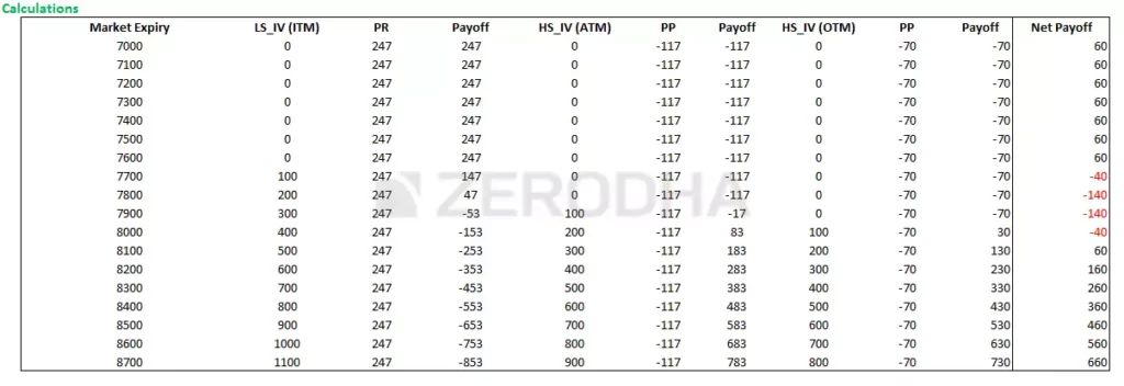
Let’s use the Nifty Spot at 7506 as an example. You predict that Nifty will reach 7000 by expiration. This is unmistakably a pessimistic expectation. The Put Ratio Back Spread should be used if:
- Sell one lot of 7500 PE (ITM)
- Buy two lots of 7200 PE (OTM)
Make sure –
- The Put options belong to the same expiry
- Belong to the same underlying
- The ratio is maintained
The trade set up looks like this –
- 7500 PE, one lot short, the premium received for this is Rs.134/-
- 7200 PE, two lots long, the premium paid is Rs.46/- per lot, so Rs.92/- for 2 lots
- Net Cash flow is = Premium Received – Premium Paid i.e 134 – 92 = 42 (Net Credit)
Situation 1: The market closes at 7600 (above the ITM option)
Both Put options would expire worthless at 7600. Following are the intrinsic value of options and the ultimate strategy payoff:
7500 PE would also expire worthless, but we have written this option and received a premium of Rs.134, which in this case can be retained back. 7200 PE would also expire worthless, but since we are long 2 lots of this option at a cost of Rs.46 per lot, we would lose the entire premium of Rs.92 paid.
134 – 92 = 42 is the strategy’s net payoff.
Keep in mind that the strategy’s net payoff at 7600 (higher than the ITM strike) is equal to the net credit.
The market expires in scenario 2 at 7,500. (at the higher strike i.e the ITM option)
Both options would expire worthless at 7500 because neither would have any intrinsic value. As a result, the reward would be comparable to the reward we discussed at 7600. As a result, the net strategy payoff would be Rs. 42. (net credit).
In actuality, as you might have guessed, the strategy’s payoff at any point above 7500 equals the net credit.
The entire premium paid, or $92, will be lost because the 7200 PE has no intrinsic value.
Therefore, we would lose 92 on the 7200 PE while making 92 on the 7500 PE, resulting in no loss and no gain. As a result, one of the breakeven points is 7458.
Scenario 4 – Market expires at 7200 (Point of maximum pain)
This is the point at which the strategy causes maximum pain, let us figure out why.
- At 7200, 7500 PE would have an intrinsic value of 300 (7500 – 7200). Since we have sold this option and received a premium of Rs.134, we would lose the entire premium received and more. The payoff on this would be 134 – 300 = – 166
- 7200 PE would expire worthless as it has no intrinsic value. Hence the entire premium paid of Rs.92 would be lost
- The net strategy payoff would be -166 – 92 = – 258
- This is a point where both the options would turn against us, hence is considered as the point of maximum pain
5.3 – Strategy Generalization
Based on the scenarios discussed above, we can draw a few conclusions:
Technically speaking, this is a ladder and not a spread. The first two option legs, however, produce a traditional “spread” in which we sell ITM and buy ATM. It is possible to interpret the spread as the difference between ITM and ITM options. It would be 200 in this instance (7800 – 7600).
Net Credit equals Premium collected from ITM CE minus Premium paid to ATM and OTM CE
Spread (difference between the ITM and ITM options) – Net Credit equals the maximum loss.
When ATM and OTM Strike, Max Loss occurs.
When the market declines, the reward equals Net Credit.
Lower Strike plus Net Credit equals Lower Breakeven.
Upper Breakeven is equal to the sum of the long strike, short strike, and net premium.
Take note of how the strategy loses money between 7660 and 8040 but ends up profiting greatly if the market rises above 8040. You still make a modest profit even if the market declines. However, if the market does not move at all, you will suffer greatly. Because of the Bear Call Ladder’s characteristics, I advise you to use it only when you are positive that the market will move in some way, regardless of the direction.
In my opinion, when the quarterly results are due, it is best to use stocks (rather than an index) to implement this strategy.
5.4 – Effect of Greeks
I assume you are already familiar with these graphs. The following graphs demonstrate the profitability of the strategy taking into account the time until expiration; as a result, these graphs assist the trader in choosing the appropriate strikes.
The best strikes to choose are deep ITM and slightly ITM, i.e., 7600 (lower strike short) and 7900, if you expect the move during the second half of the series and you expect it to happen within a day (or within 5 days, graph 2). (higher strike long). Please take note that this is an ITM and ITM spread rather than the traditional combination of an ITM + OTM spread. In actuality, none of the other combinations work.
Graphs 3 (bottom right) and 4 (bottom left): The best strategy is to use these graphs if you anticipate a move during the second half of the series and that it will occur within 10 days (or on the expiry day, graph 4).Deep ITM and slightly ITM strikes, such as 7600 (lower strike short) and 7900, are the best options (higher strike long). This is in line with what graphs 1 and 2 indicate.
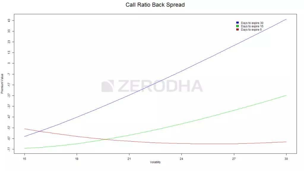
The relationship between the change in “premium value” and the change in volatility is shown by three coloured lines. These lines make it easier for us to comprehend how an increase in volatility affects the strategy while keeping the time until expiration in mind.
Green line – This line suggests that, although not as much as in the preceding case, an increase in volatility is advantageous when there are roughly 15 days until expiration. As we can see, when volatility rises from 15% to 30%, the strategy payoff increases from -77 to -47.
Red line: Clearly, the premium value is not significantly affected by an increase in volatility as time approaches expiration. This indicates that when expiration is approaching, you should only be concerned with directional movement and not much with volatility variation.
For Visit: Click here to know the directions.