Bear put spread
Basics of stock market
• Induction
• Bull call spread
• Bull put spread
• Call ratio Back Spread
• Bear call ladder
• Synthetic long & Arbitrage
• Bear put spread
• Bear call spread
• put ration back spread
• Long straddle
• Short straddle
• Max pain & PCR ratio
• Iron condor
7.1 – Spreads versus naked positions
Over the last five chapters, we’ve discussed various multi-leg bullish strategies. These strategies ranged to suit an assortment of market outlooks – from an outrightly bullish market outlook to a moderately bullish market outlook.
Reading through the last 5 chapters you must have realized that most professional options traders prefer initiating a spread strategy versus taking on naked option positions. No doubt spreads tend to shrink the overall profitability, but at the same time spreads give you greater visibility on risk. Professional traders value ‘risk visibility’ more than profits. In simple words, it’s a much better deal to take on smaller profits as long as you know what would be your maximum loss under worst-case scenarios.
Spreads have another intriguing feature in that there is always some form of financing involved, with the sale of one option funding the purchase of another. In actuality, one of the primary characteristics that set a spread apart from a typical naked directional position is financing. The strategies you can use when your outlook is neutral to strongly negative will be covered in the following chapters. These strategies share characteristics with the bullish strategies that we covered earlier in the module.
The Bear Put Spread, which is, as you might have guessed, the inverse of the Bull Call Spread, is the first bearish strategy we’ll examine.

4.2 – Strategy Notes
The Bear Put Spread is similarly simple to use as the Bull Call Spread. When the market outlook is moderately bearish,
that is, when you anticipate that the market will decline in the short term but not significantly, you would use a bear put spread. A correction of 4-5 percent would be appropriate if I were to quantify what “moderately bearish” means.
If the markets are correct as anticipated (go down), one would make a modest profit by using a bear put spread; however,
if the markets go up, the trader would only suffer a small loss.
A conservative trader (read as a risk-averse trader) would implement the Bear Put Spread strategy by simultaneously –
Buying an In the money Put option
Selling an Out of the Money Put option
The creation of an ITM and OTM option for the Bear Put Spread is not required. Any two put options can be used to create the bear put spread. The trade’s level of aggression affects the strike decision. But keep in mind that both options must have the same expiration date and underlying. Let’s look at an example and various scenarios to see how the strategy operates in order to better understand the implementation.
Nifty is currently trading at 7485, which means that 7600 PE is in the black and 7400 PE is out of the money.
To use the “Bear Put Spread,” one would have to sell the 7400 PE, and the premium they would receive from doing so would help to pay for the 7600 PE.
In relation to the 7600 PE, the premium received (PR) is Rs. 73, and the premium paid (PP) is Rs. 165.
This transaction’s net debit would be –
We need to take into account various scenarios in order to comprehend how the strategy’s payoff functions under various expiry conditions. Please keep in mind that the payoff occurs at expiration, which means that the trader must hold these positions until expiration.
Situation 1: The market closes at 7800 (above long put option i.e 7600)
In this instance, the market has increased despite expectations that it would decline. Both of the put options at 7800, 7600, and 7400, would have no intrinsic value and would therefore expire worthlessly.
We would keep nothing because the premium we paid for 7600 PE, which was Rs. 165, would become 0.
The premium for the 7400 PE, or Rs. 73, would be kept in full.
Therefore, at 7800, we would experience a loss of Rs. 165 on the one hand, but this would be partially offset by the premium received, which is Rs. 73.
-165 + 73 = -92 would be the total loss.
Please take note that the ‘-ve’ sign next to 165 denotes a money outflow from the account, while the ‘+ve’ sign next to 73 denotes a money inflow into the account.
Additionally, the strategy’s net debit is equal to the strategy’s net loss of 92.
Scenario 2 – Market expired at 7600 (at long put option)
Here, we’ll assume that the market expires at 7600, the price at which we bought the Put option.
Then, at 7600, both the PE for 7600 and the PE for 7400 would expire worthless (similar to scenario 1),
resulting in a loss of -92.
Scenario 3 – Market expires at 7508 (breakeven)
7508 is halfway through 7600 and 7400, and as you may have guessed I’ve picked 7508 specifically to showcase that the strategy neither makes money nor loses any money at this specific point.
The 7600 PE would have an intrinsic value equivalent to Max [7600 -7508, 0], which is 92.
Since we have paid Rs.165 as a premium for the 7600 PE, some of the premium paid would be recovered. That would be 165 – 92 = 73, which means to say the net loss on 7600 PE at this stage would be Rs.73 and not Rs.165
The 7400 PE would expire worthlessly, hence we get to retain the entire premium of Rs.73
So on hand, we make 73 (7400 PE) and on the other, we lose 73 (7600 PE) resulting in a no loss no profit situation
Hence, 7508 would be the breakeven point for this strategy.
Scenario 4 – Market expires at 7400 (at short put option)
This is an interesting level, do recall when we initiated the position the spot was at 7485, and now the market has gone down as expected. At this point, both options would have interesting outcomes.
The 7600 PE would have an intrinsic value equivalent to Max [7600 -7400, 0], which is 200
We have paid a premium of Rs.165, which would be recovered from the intrinsic value of Rs.200, hence after compensating for the premium paid one would retain Rs.35/-
The 7400 PE would expire worthlessly, hence the entire premium of Rs.73 would be retained
The net profit at this level would be 35+73 = 108
The net payoff from the strategy is in line with the overall expectation from the strategy i.e the trader gets to make a modest profit when the market goes down.
Situation 5: The market closes at 7200 (below the short put option)
Again, this is an intriguing level because both possibilities would be valuable in and of themselves.
Let’s determine whether the numbers add up.
The intrinsic value of the 7600 PE would be equal to Max [7600 -7200, 0], which is 400.
After paying back the premium of Rs. 165 that we paid, which would be recovered from the intrinsic value of Rs. 400,
one would still be left with Rs. 235.
The intrinsic value of the 7400 PE would be Max [7400 -7200, 0], which is 200.
We were given a premium of Rs. 73, but we will have to forfeit it and take a loss in excess of Rs. This equals 200 – 73.
7.3 – Strategy critical levels
From the scenarios discussed above, we can generalize the following:
If the spot moves above the breakeven point, the strategy loses money, and if it moves below the breakeven point,
it makes money.
The profits and losses are both limited.
The spread is the variation in the two strike prices.
Spread in this case would be 7600 – 7400 = 200.
Net Debit = Premium Paid – Premium Received, which is 165 – 73, to equal 92.
Higher strike – Net Debit 7600 – 92 = 7508 is the breakeven point.
Max profit is equal to Spread – Net Debit (200 – 92) (108).
Maximum Loss = 92 Net Debit
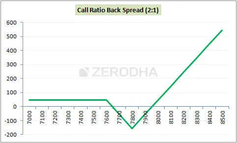
All of these crucial details can be seen in the strategy payoff diagram:
7.4 – Quick note on Delta
It’s better late than never: I should have included this in the earlier chapters. Every time you use an options strategy, add up the deltas. I calculated the deltas using the B&S calculator.
7600 PE’s delta is -0.618.
-(-0.342)
+ 0.342
Now, since deltas are additive in nature we can add up the deltas to give the combined delta of the position. In this case,
it would be –
-0.618 + (+0.342)
= – 0.276
The ‘-ve’ denotes that the premiums will increase if the markets decline, giving the strategy an overall delta of 0.276.
Similar to the Bull Call Spread, Call Ratio Back spread, and other strategies we’ve discussed in the past, you can add up their deltas and see that they all have a positive delta, indicating that the strategy is bullish.
It becomes very challenging to determine the overall bias of the strategy—whether it is bullish or bearish—when there are more than two option legs. In these situations, you can quickly add up the deltas to determine the bias. Additionally, if the sum of the deltas to zero, the strategy is not particularly biased in any direction.
7.5 – Strike selection and effect of volatility
The strike selection for a bear put spread is very similar to the strike selection methodology of a bull call spread.
0 I hope you are familiar with the ‘1st half of the series’ and ‘the 2nd half of the series methodology. If not I’d suggest you kindly read through section 2.3.
Have a look at the graph below –
Choose the following strikes to create the spread if we are in the first half of the series (ample time before expiry) and anticipate a market decline of about 4% from current levels:
The premium varies according to changes in volatility and time, as shown in the graph above.
The blue line indicates that when there is enough time before expiration, the cost of the strategy does not change significantly with the rise in volatility (30 days)
When there are roughly 15 days until expiration, the green line indicates that the cost of the strategy varies moderately
with the rise in volatility.
The red line indicates that with approximately 5 days until expiration, the cost of the strategy varies significantly with the rise in volatility.
These graphs make it obvious that when there is enough time before expiration, one shouldn’t worry too much about changes in volatility. However, one must possess a view of the volatility between the series’ midpoint and its expiration. Only use the bear put spread if you anticipate an increase in volatility; otherwise, avoid using the strategy if you anticipate a decrease in volatility.
4.3 – Strategy Generalization
Going by the above-discussed scenarios we can make a few generalizations –
- Spread = Higher Strike – Lower Strike
- Net Credit = Premium Received for lower strike – 2*Premium of higher strike
- Max Loss = Spread – Net Credit
- Max Loss occurs at = Higher Strike
- The payoff when the market goes down = Net Credit
- Lower Breakeven = Lower Strike + Net Credit
- Upper Breakeven = Higher Strike + Max Loss
Here is a graph that highlights all these important points –
4.4 – Welcome back the Greeks
I assume you are already familiar with these graphs. The following graphs demonstrate the profitability of the strategy taking into account the time until expiration; as a result, these graphs assist the trader in choosing the appropriate strikes.
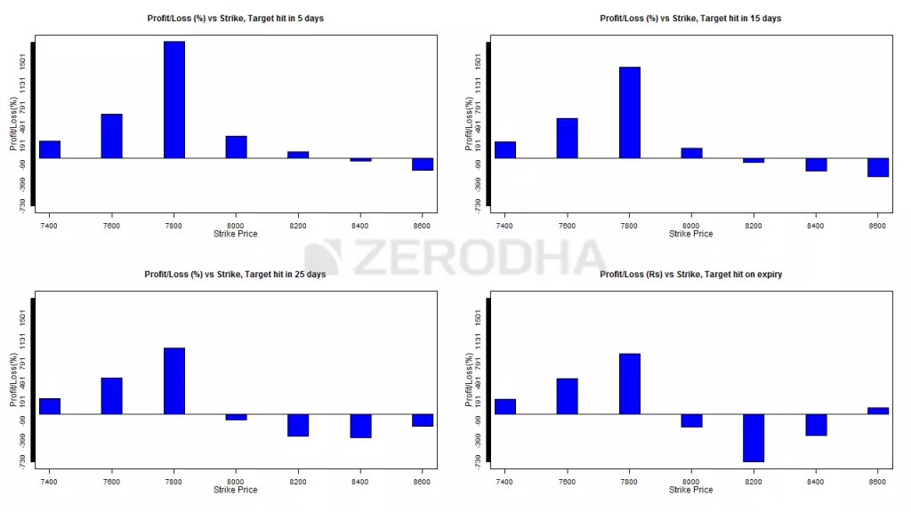
Before understanding the graphs above, note the following –
-
The nifty spot is assumed to be at 8000
-
The start of the series is defined as any time during the first 15 days of the series
-
The end of the series is defined as any time during the last 15 days of the series
-
The Call Ratio Back Spread is optimized and the spread is created with 300 points difference
The market is predicted to increase by about 6.25 percent, or from 8000 to 8500. In light of the move and the remaining time, the graphs above indicate that –
Top left on Graph 1 and top right on Graph 2 – The most profitable strategy is a call ratio spread using 7800 CE (ITM) and 8100 CE (OTM), where you would sell 7800 CE and buy 2 8100 CE. This is because you are at the beginning of the expiry series and you anticipate the move over the next 5 days (and 15 days in the case of Graph 2) Do keep in mind that even though you would be correct about the movement’s direction, choosing other far OTM strikes call options usually results in losses.
Graphs 3 and 4 (bottom left and bottom right, respectively) – A Call Ratio Spread using 7800 CE (ITM) and 8100 CE (OTM) is the most profitable option if you are at the beginning of the expiry series and anticipate the move in 25 days (and expiry day in the case of Graph 3). In this scenario, you would sell 7800 CE and buy 2 8100 CE.
You must be wondering why the number of strikes is the same regardless of the time remaining. In fact, this is the key: the call ratio back spread functions best when you sell slightly ITM options and buy slightly OTM options with plenty of time left before expiration. In actuality, all other combinations are in the red, particularly those that include far OTM options.
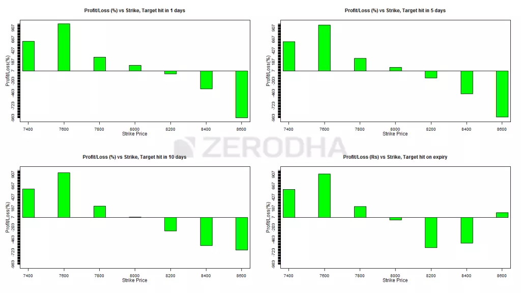
The best strikes to choose are deep ITM and slightly ITM, i.e., 7600 (lower strike short) and 7900, if you expect the move during the second half of the series and you expect it to happen within a day (or within 5 days, graph 2). (higher strike long). Please take note that this is an ITM and ITM spread rather than the traditional combination of an ITM + OTM spread.
In actuality, none of the other combinations work.
Graphs 3 (bottom right) and 4 (bottom left): The best strategy is to use these graphs if you anticipate a move during the second half of the series and that it will occur within 10 days (or on the expiry day, graph 4). Deep ITM and slightly ITM strikes, such as 7600 (lower strike short) and 7900, are the best options (higher strike long). This is in line with what graphs 1 and 2 indicate.
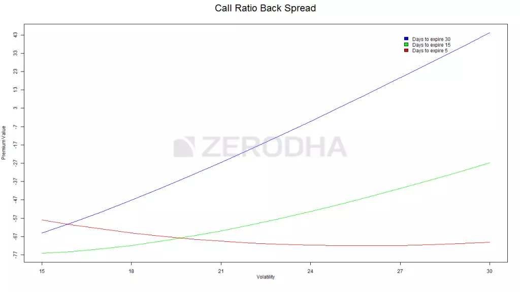
Three colored lines show the relationship between the change in “net premium,” or the strategy payoff, and the change in volatility. These lines give us insight into how an increase in volatility affects the strategy while keeping the time until expiration in perspective.
The blue line indicates that a rise in volatility with plenty of time left before expiration (30 days) is advantageous for the
call ratio back spread. As we can see, when volatility rises from 15% to 30%, the strategy’s payoff increases from -67 to +43. This obviously implies that when there is enough time before expiration, in addition to being accurate about the direction of the stock or index, you also need to have a view of volatility. Because of this, even though I believe the stock will rise, I would be a little hesitant to use this strategy at the beginning of the series if volatility is higher than average (say more than double the usual volatility reading)
Green line – This line suggests that, although not as much as in the preceding case, an increase in volatility is advantageous when there are roughly 15 days until expiration. As we can see, when volatility rises from 15% to 30%, the strategy payoff increases from -77 to -47.
Red line: This result is intriguing and illogical. The strategy is negatively impacted by an increase in volatility when there are only a few days left until expiration! Consider that a rise in volatility near the expiration date increases the likelihood that the option will expire in the money, which lowers the premium. So, if you are bullish on a stock or index with a few days left until expiration and you anticipate that volatility will rise during this time, proceed with caution.
For Visit: Click here to know the directions.