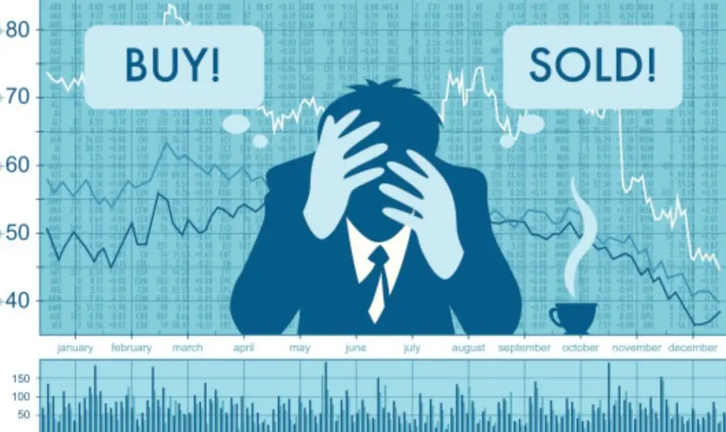
For traders and investors who want to successfully navigate the intricate world of financial markets in today’s fast-paced financial environment, learning the art of technical trading is imperative. We have developed this extensive guide to help you outrank the current article on “What is the best technical trading?” and give you the knowledge you need to succeed in technical trading. We are specialists in SEO and premium copywriting.
Introduction to Technical Trading
Technical traders use technical analysis, another name for technical trading, to predict future price movements based on volume, past price data, and other market statistics. This strategy is based on the idea that past trading data can offer insightful information about potential future trends in the market.
Key Concepts of Technical Trading
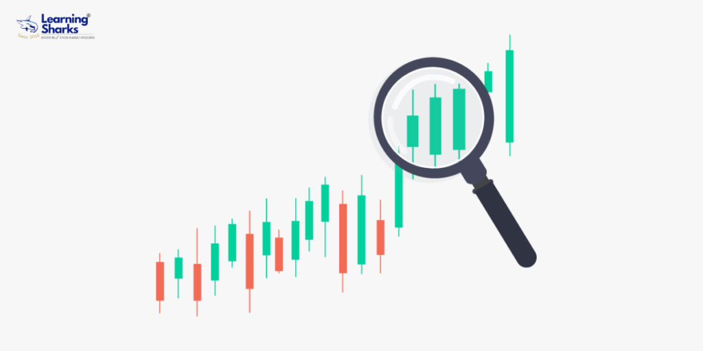
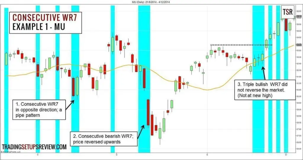
- Candlestick Patterns
Knowing candlestick patterns is one of the core concepts of technical trading. Understanding how to interpret these patterns—which show an asset’s price movements—is essential to making wise trading decisions. Some typical candlestick patterns are as follows: - Support and Resistance Levels
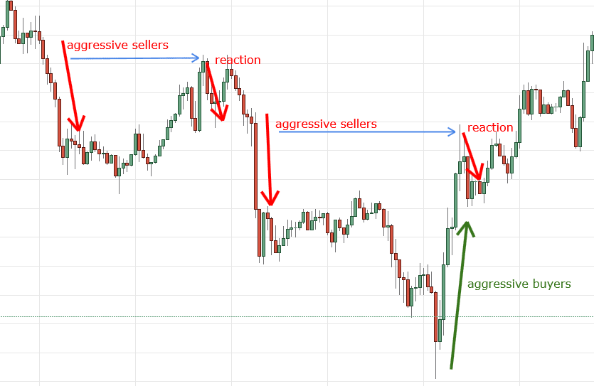
In technical trading, support and resistance levels are crucial. Resistance denotes a price point at which selling interest usually appears, whereas support denotes a price point at which an asset typically finds buying interest. These levels are used by traders to determine possible entry and exit points.
Technical Trading Tools
You must use a variety of tools and indicators to help you analyze price trends and market sentiment if you want to succeed at technical trading.
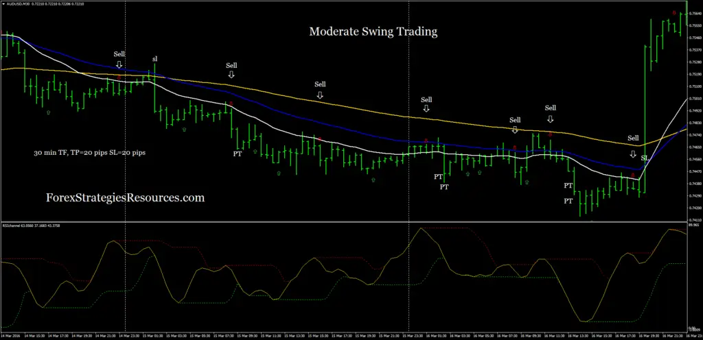
1. Moving Averages
Moving averages are crucial instruments for taming price data so that trends over a given time span can be identified. Two typical kinds are:
- Simple Moving Average (SMA): Gives a clear average of prices over a selected period of time.
- Exponential Moving Average (EMA): Increases the weight given to recent prices, increasing its responsiveness to changes in prices recently.
2. Relative Strength Index (RSI)
A momentum oscillator that gauges the velocities and variations in price movements is the RSI. It detects overbought and oversold situations by oscillating between 0 and 100.
Technical Trading Strategies
Technical analysis requires well-defined trading strategies to be used effectively.
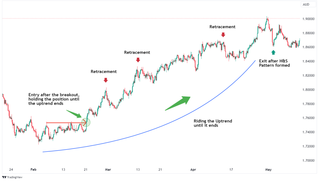
- Trend Following
Trading in the direction of recognized price trends is the goal of trend following strategies. Traders can identify these trends by using trendlines or moving averages. - Breakout Trading
The goal of breakout trading is to profit from large price shifts that occur after a period of range-bound or consolidation trading. To find possible breakout opportunities, traders search for important levels of support and resistance. - Support and Resistance Trading
Buying at support levels and selling at resistance levels are the cornerstones of this strategy. At these times, traders wait for price reversals before acting.
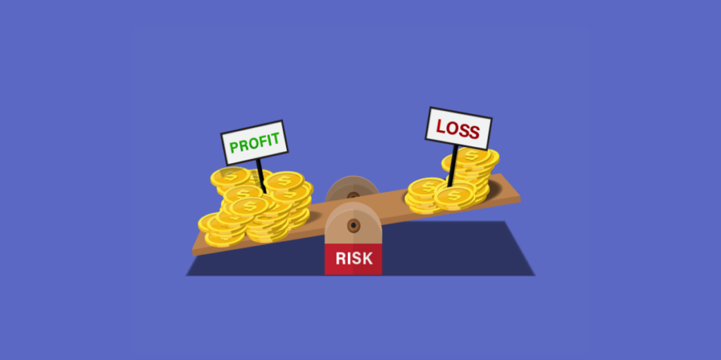
Risk Management in Technical Trading
In technical trading, risk management must be done effectively. The best of strategies can lead to large losses if risk management is not properly managed. Setting stop-loss orders, diversifying your holdings, and never taking on more risk than you can afford to lose are all very important.
Conclusion
To sum up, technical trading is an effective strategy for negotiating the intricacies of the financial markets. You can improve your trading abilities and make wise investment decisions by learning how to read candlestick patterns, applying fundamental technical tools and strategies, and comprehending support and resistance levels.
FOR MORE INFO CLICK THIS SITE:https://learningsharks.in/
FOLLOW OUR PAGE:https://www.instagram.com/learningsharks/?hl=en