top 10 stock exchange in the world
1.The New York Stock Exchange (NYSE) in the US
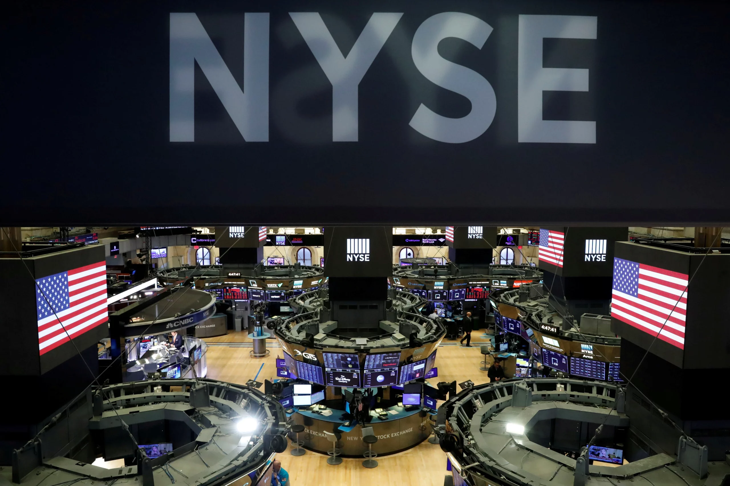
Market value: More than $30 trillion
Established in 1792; based in New York City, United States.
Among those companies listed on the New York Stock Exchange are many of the world’s largest companies, including foreign companies across various industries.
The NYSE trading floor is housed in the New York Stock Exchange building, which is on the national historic properties list. It is located at 11 Wall Street and 18 Broad Street. The historic trading room at 30 Broad Street was closed in February 2007. The NYSE’s opening and closing bells signal the start and finish of each trading day. The opening bell rings at 9:30 a.m. ET to signal the start of the day’s trading session. At 4 p.m. ET, the closing bell rings, and trading for the day comes to an end. When a button is touched, bells in each of the NYSE’s four main sections ring simultaneously.
2..National Association of Securities Dealer Automatic Quotation (NASDAQ)

Market value: More than $22 trillion
Founded in 1971 and based in New York City, USA.
The NASDAQ is the world’s second-largest stock exchange by market capitalization and boasts a high technology content. Additionally, the US-based exchange was the world’s first electronic stock market. In 1992, the Nasdaq Stock Market and the London Stock Exchange formed the first intercontinental connectivity of financial markets.
3.Tokyo Stock Exchange (TSE) of Japan
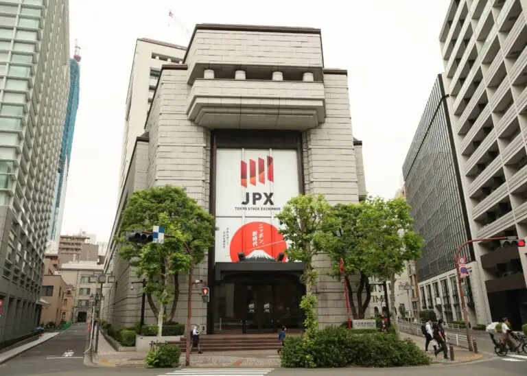
Market value: More than $6 trillion
Established in 1878; Headquarters in Tokyo, Japan
One of the world’s finest stock exchanges is in Tokyo, Originally established in 1878, it was a trading platform for newly issued government bonds to former samurai.
A pre-opening auction will take place from 9:00 to 9:30 a.m. The opening price of a securities is announced shortly after 9:20 a.m. A morning trading session from 9:30 a.m. until 12:00 p.m. A prolonged morning session from 12:00 noon to 1:00 pm, often known as lunch break.[19][20] Continuous trading occurs in precisely specified assets (currently two ETFs, 4362 and 4363). It is not feasible to trade other securities. However, already made orders in any securities can be canceled beginning at 1:00 p.m.
An afternoon continuous trading session runs from 1:00 to 4:00 p.m. The closing price is calculated by using the median of five price snapshots every 15 seconds between 3:59 and 4:00 p.m.
4.China’s Shanghai Stock Exchange(SSE)
Market value: More than $5 trillion
Established: 1990
Where: Shanghai China
With a sizable number of Chinese state-owned businesses and private sector companies, the SSE is one of the biggest stock exchanges in Asia and the globe. The SSE is available for trade Monday through Friday from 09:15 to 15:00. The morning session begins with centralized competitive pricing from 09:15 to 09:25, followed by successive bidding from 09:30 to 11:30. This is followed by an afternoon continuous bidding session that runs from 13:00 to 14:57. The centralized competitive pricing resumes from 14:57 to 15:00, and block trading continues from 15:00 to 15:30. The market is closed on Saturday and Sunday, along with other holidays stated by the SSE.
5. Euronext Stock Exchange:
Market value: approximately $5 trillion
Established in 2000 with headquarters in Amsterdam, Netherlands, with marketplaces in Paris, Brussels, Lisbon, Dublin, and Oslo Euronext is a pan-European stock market organization that lists numerous top international corporations and includes several key European countries.
6. Hong Kong's Hong Kong Stock Exchange (HKEX)
Market Value: More than $4 trillion
Established: 1891
Where: Hong Kong
One of Asia’s main financial centers, the HKEX is home to numerous Chinese and foreign businesses. A trading day consists,
Depending on market performance and worldwide economic conditions, these rankings may change over time. Nonetheless, in terms of market capitalization and importance, the aforementioned exchanges have continuously been among the best.
7. The UK's London Stock Exchange (LSE)
About $ 4 trillion is the market capitalization.
Established: 1801
Where: London, UK
One of the world’s oldest and most prominent stock exchanges, the LSE lists a variety of multinational corporations.
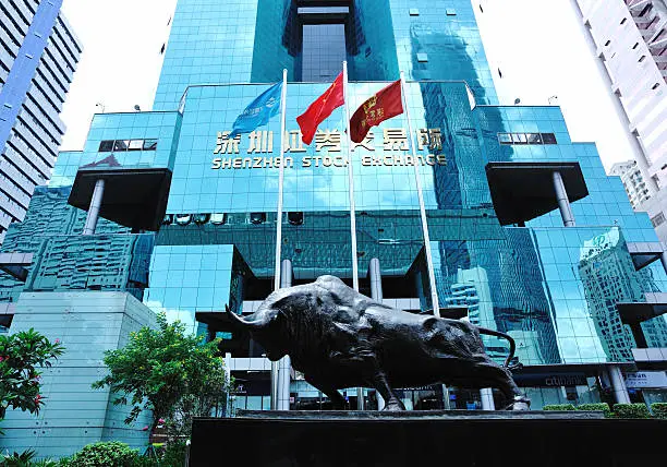
8. China's Shenzhen Stock Exchange (SZSE)
Market Value: More than $4 trillion
Established: 1990Location: China’s Shenzhen
A vital component of China’s financial system, the SZSE focuses on innovation, technology, and smaller businesses.
9. Canada's Toronto Stock Exchange (TSX)
About $3 trillion is the market capitalization.
Established: 1852
Where: Toronto, Canada
The largest stock exchange in Canada, the TSX, is home to many resource-based businesses, especially those in the mining and energy sectors.
10. India's National Stock Exchange (NSE)

About $3 trillion is the market.
Established: 1992
Where: Mumbai, India
Many Indian and international companies are based on the NSE, which is the biggest stock exchange in India in terms of market capitalization and volume.
Conclusion
These top stock markets illustrate the global economy’s diversity and complexity, with each providing distinct possibilities for investors. From established US markets to rising Asian exchanges, these markets provide access to a variety of geographies, sectors, and growth phases, balancing economic stability with growth potential. Understanding these exchanges is critical for investors seeking to develop a globally diversified portfolio, leveraging on economic strengths, and minimizing regional risks.