Greek Calculator

September 21, 2022August 4, 2022 by Rohansharma

Options

• Basics of call options
• Basics of options jargon
• How to buy a call option
• How to buy/sell call option
• Buying put option
• Selling put option
• Call & put options
• Greeks & calculator

• Option contract
• The option greeks
• Delta
• Gamma
• Theta
• All volatility
• Vega

21.1 – Background

We have already covered all the significant Option Greeks and their applications in this module. It’s time to comprehend how to use the Black & Scholes (BS) Options pricing calculator to calculate these Greeks. The Black and Scholes options pricing model, from which the name Black & Scholes derives, was first published by Fisher Black and Myron Scholes in 1973. Robert C. Merton, however, developed the model and added a complete mathematical understanding to the pricing formula.

Because of how highly regarded this pricing model is in the financial world, Robert C. Merton and Myron Scholes shared the 1997 Nobel Prize in Economic Sciences. Mathematical concepts like partial differential equations, the normal distribution, stochastic processes, etc. are used in the B&S options pricing model. This module’s goal is not to walk you through the math in the B&S model; instead, you should watch this Khan Academy video.

21.2 – Overview of the model

Consider the BS calculator as a “black box,” which accepts a variety of inputs and produces a variety of outputs. The majority of the market data for the options contract must be provided as inputs, and the outputs are the Option Greeks.

This is how the pricing model’s framework operates:

Spot price, strike price, interest rate, implied volatility, dividend, and the number of days until expiration are the inputs we give the model.
The pricing model generates the necessary mathematical calculation and outputs a number of results.

The output includes all Option Greeks as well as the call and put option’s theoretical price for the chosen strike.
The schematic of a typical options calculator is shown in the following illustration:

The spot price at which the underlying is trading is known as the spot price. Note that we can even substitute the futures price for the spot price. When the underlying of the option contract is a futures contract, we use the futures price. The currency options and the commodity options are frequently based on futures. Utilize the spot price exclusively for equity option contracts.

Interest Rate: This is the market-prevailing, risk-free rate. For this, use the RBI’s 91-day Treasury bill rate. The rate is available on the RBI website’s landing page, which is highlighted in the example below.

Dividend – This is the anticipated dividend per share for the stock, assuming it goes ex-dividend during the expiration period. Assume, for instance, that you want to determine the Option Greeks for the ICICI Bank option contract as of today, September 11th. Consider that ICICI Bank will begin paying a dividend of Rs. 4 on September 18th. Since the September series expires on September 24, 2015, the dividend in this instance would be Rs. 4.

Days remaining before expiration – This is the remaining number of calendar days.

Volatility: You must enter the implied volatility of the option here. You can always extract the implied volatility information by looking at the option chain that NSE provides. Here is an illustration of a snap.

Let’s use this knowledge to determine the ICICI 280 CE option Greeks.

Price at Spot = 272.7

Interest rate equals 7.4769 %

Division = 0

Days until expiration = 1 (today is 23rd September, and expiry is on 24th September)

Volatility is equal to 43.55%

We must enter this data into a typical Black & Scholes Options calculator once we have it. You can calculate the Greeks using the calculator found on our website at https://zerodha.com/tools/black-scholes.

Note the following on the output side:

Calculated is the premium for 280 CE and 280 PE. According to the B&S options calculator, this is the theoretical option price. Ideally, this should coincide with the market’s current option price.

All of the Options Greeks are listed below the premium values.

I’m assuming that by this point you are fairly familiar with the meanings and applications of each Greek word.

One last thing to remember about option calculators: they are primarily used to figure out the Option Greeks and the theoretical option price. Due to differences in input assumptions, minor differences can occasionally occur. It is advantageous to allow for the inescapable modelling errors for this reason. But generally speaking, the

21.3 – Put Call Parity

While we are discussing the topic on Option pricing, it perhaps makes sense to discuss ‘Put Call Parity’ (PCP). PCP is a simple mathematical equation which states –

Put Value + Spot Price = Present value of strike (invested to maturity) + Call Value.

The equation above holds true assuming –

Both the Put and Call are ATM options
The options are European
They both expire at the same time
The options are held till expiry

For people who are not familiar with the concept of Present value, I would suggest you read through this – http://zerodha.com/varsity/chapter/dcf-primer/ (section 14.3).

Assuming you are familiar with the concept of Present value, we can restate the above equation as –

P + S = Ke^(-rt) + C

Where, Ke^(-rt) represents the present value of strike, with K being the strike itself. In mathematical terms, strike K is getting discounted continuously at rate of ‘r’ over time‘t’

Also, do realize if you hold the present value of the strike and hold the same to maturity, you will get the value of strike itself,

hence the above can be further restated as –

Put Option + Spot Price = Strike + Call options

Why then should the equality persist? Think about two traders, Trader A and Trader B, to help you better understand this.

A trader holds an ATM. 1 share of the underlying stock and a put option (left hand side of PCP equation)

Trader B is in possession of a call option and cash equal to the strike (right hand side of PCP equation)

Given this situation, both traders should profit equally under the PCP (assuming they hold until expiry). Let’s enter some data to assess the equation:

Underlying = Infosys
Strike = 1200
Spot = 1200

Trader A holds = 1200 PE + 1 share of Infy at 1200
Trader B holds = 1200 CE + Cash equivalent to strike i.e 1200

Assume upon expiry Infosys expires at 1100, what do you think happens?

Trader A’s Put option becomes profitable and he makes Rs.100 however he loses 100 on the stock that he holds, hence his net pay off is 100 + 1100 = 1200.

Trader B’s Call option becomes worthless, hence the option’s value goes to 0, however he has cash equivalent to 1200, hence his account value is 0 + 1200 = 1200.

Let’s take another example, assume Infy hits 1350 upon expiry, lets see what happens to the accounts of both the trader’s.

Trader A = Put goes to zero, stock goes to 1350/-
Trader B = Call value goes to 150 + 1200 in cash = 1350/-

So it is obvious that the equations hold true regardless of where the stock expires, resulting in the same amount of profit for both traders A and B.

All right, but how would you create a trading strategy using the PCP? You’ll have to wait until the next module, which is about “Option Strategies,” to find out, J. There are still two chapters left in this module before we begin the module on option strategies.

Buying put option

August 4, 2022 by Bala gumber

Options

• Option contract
• The option greeks
• Delta
• Gamma
• Theta
• All volatility
• Vega

5.1 – Getting the orientation right

I hope you’ve finished thinking about the call option’s realities from both the sellers’ and buyers’ points of view. If you are familiar with call options, it will be quite simple for you to grasp “put options.” From the standpoint of the buyer, the only difference between a put option and a call option is that the put option buyer should have a negative opinion of the markets as opposed to an optimistic view.

The purchaser of the put option is placing a wager that the stock price will decline (by the time expiry approaches). He, therefore, gets into a Put Option arrangement in order to profit from this viewpoint.

No matter where the underlying stock is trading, the buyer of a put option can purchase the right to sell a stock at a price (the striking price) under a put option agreement.

Keep in mind this generalization: Since the seller of the option expects the exact opposite of what the buyer does, there is a market. A market cannot exist if everyone has the same expectations. Therefore, the put option seller would anticipate a rise in the market (or a flattening of the stock) if the put option buyer anticipates a decline by expiration.

At a set price (the strike price), a put option buyer purchases the put option writer’s right to sell the underlying. This indicates that if the “put option buyer” is selling the put option seller, he will have to buy at expiration. Keep in mind that the put option seller is actually selling the put option buyer a right to “sell” the underlying to the “put option seller” at the time of expiration at the time of the agreement.

Confusing? Consider the “Put Option” as a straightforward agreement between two parties to conduct a transaction based on the price of an underlying –

The parties involved in a contract are referred to as the “contract buyer” and the “contract seller,” respectively.
The contract buyer invests money and purchases a right for himself.
The contract seller accepts the premium and commits to the deal.
On the day of expiration, the contract buyer will choose whether or not to exercise his right.
The contract seller is bound to purchase the underlying from the contract buyer if the contract buyer decides to exercise his right and sells the underlying (which may be a stock) at the agreed-upon price (the striking price).
Since the contract the buyer holds allows him to sell the underlying at a much higher price to the contract seller when the same underlying is trading at a lower price in the open market, it stands to reason that the contract buyer will only exercise his right if the underlying price is trading below the strike price.

Still perplexing? Do not be alarmed; an example will be used to help you better comprehend this.

Take into account the following scenario between the Contract seller and the Contract buyer:

Consider that Reliance Industries is currently trading at Rs. 850.
The contract buyer pays the contract seller Rs. 850 for the opportunity to purchase Reliance when it expires.
The contract buyer must pay a premium to the contract seller in order to secure this entitlement.
The contract seller will agree to purchase Reliance Industries shares at Rs. 850 a share in exchange for the premium, but only if the contract buyer wants him to purchase them from him.
For instance, if Reliance is trading at Rs. 820 upon expiration, the contract buyer may demand that the contract seller purchase Reliance from him for Rs. 850.
This indicates that the contract buyer can earn from selling Reliance for Rs. 850/- even if it is currently trading at Rs. 820/- on the open market.
It makes no sense for the contract buyer to exercise his right and ask the contract seller to acquire the shares from him at Rs. 850/- if Reliance is trading at Rs. 850/- or more upon expiration (let’s say Rs. 870/-). Given that he can sell it for more money on the open market, this is rather clear.
A “Put option” is a contract of this type that grants the buyer the right to sell the underlying asset when it expires.
Due to his sale of the contract buyer’s Reliance 850 Put Option, the contract seller will be required to purchase Reliance at Rs. 850.

I hope the discussion above has provided you with the necessary introduction to put options. It’s okay if you’re still unclear because as we move forward, I’m sure you’ll become more understandable. However, there are three crucial things you should know right now:

The put option’s seller is neutral or optimistic about the underlying asset, whereas the put option’s buyer is gloomy about it.
When the put option expires, the buyer has the opportunity to sell the underlying asset for the strike price.
Due to receiving an upfront premium, the put option seller is required to purchase the underlying asset from the put option buyer at the strike price.

5.2 – Building a case for a Put Option buyer

Let’s construct a real-world scenario to grasp the put option better, just like we did with the call option. We will first discuss the put option from the buyer’s standpoint before comprehending the put option from the seller’s standpoint.

Here are some of my opinions regarding Bank Nifty:

Trading for Bank Nifty is at 18417.
A week ago Bank Nifty encountered resistance at 18550. (resistance level highlighted by a green horizontal line)
Since there is a price action zone at this level that is evenly spaced in time, I view 18550 as resistance (for those unfamiliar with the notion of resistance, I recommend reading about it here).
The price action zone has been indicated with blue rectangle boxes.
The RBI maintained the status quo on the monetary rates on April 7th (yesterday), leaving the major central bank rates unchanged (as you may know RBI monetary policy is the most important event for Bank Nifty)
Therefore, given the technical resistance and lack of a significant fundamental trigger, banks may not be the trend in the markets this year.
Therefore, traders could choose to sell banks and purchase something else that is in demand at the moment.
I have a bearish leaning toward Bank Nifty because of these factors.
Since the market is bullish overall and just the banking sector is bearish, shorting futures may be rather dangerous.
Using an option is best in these situations, thus purchasing a Put Option on the Bank Nifty may make sense.
Keep in mind that if you purchase a put option, you profit if the underlying declines.

With this justification, I would rather purchase the 18400 Put Option, which is currently trading at a premium of Rs. 315. Remember that in order to purchase this 18400 Put option, I must pay the necessary premium (in this example, Rs. 315/-), which will be paid to the 18400 Put option seller.

The simplest way to purchase a put option is to phone your broker and ask him to do it for you in a matter of seconds. The put option can be purchased for any stock and strike. As an alternative, you can purchase it directly via a trading platform like Zerodha Pi. Later on, we will discuss the specifics of purchasing and selling options using a trading terminal.

It would be fascinating to watch the Put Option’s P&L behavior at expiration, presuming I had purchased Bank Nifty’s 18400 Put Option. We can even draw a few conclusions from this procedure regarding the P&L behavior of a Put option.

5.3 – Intrinsic Value (IV) of a Put Option

We must comprehend how to calculate a Put option’s intrinsic value before we can generalize the Put option P&L’s behavior. I’ll assume you are familiar with the idea of intrinsic value since we discussed it in the previous chapter. The intrinsic value of an option is the amount of money the buyer would be entitled to upon the expiration of the option.

A put option’s intrinsic value is calculated significantly differently than a call option’s intrinsic value. I’ll provide the call option’s intrinsic value formula here so you can see the differences.

Spot price minus strike price is the IV (call option).

A put option’s intrinsic value is –

IV (Put Option) = Spot – Strike Price

The formula we just looked at to determine an option’s intrinsic value is only applicable on the day the option expires. The intrinsic value of an option is, however, determined differently across the series. Naturally, during the expiry, we will comprehend how to determine (and the necessity of calculating) an option’s intrinsic worth. But for the time being, all that we need to know is how to calculate the intrinsic value at expiration.

5.4 – P&L behavior of the Put Option buyer

Let’s attempt to create a table that will help us determine how much money I, the buyer of Bank Nifty’s 18400 put option, would make under the various potential spot value changes of Bank Nifty (in the spot market), keeping the concept of intrinsic value of a put option at the back of our minds. Keep in mind that Rs 315 was paid as the premium for this choice. The fact that I paid Rs. 315 will not change, regardless of how the spot value increases. This is the price I paid to purchase the Bank Nifty 18400 Put Option.

Let’s examine the P&L’s behavior and make some observations (and also make a few P&L generalizations). Set your gaze at row number 8 to serve as your reference point for the conversation above.

Buying a put option is done in order to profit from a declining price. As we can see, the profit rises as and when the spot market price falls (with reference to the strike price of 18400).

1. Generalization 1: Whenever the spot price falls below the strike price, buyers of put options benefit. In other words, only purchase a put option if you believe the underlying asset will decline.

2. The strategy begins to lose money as soon as the spot price exceeds the strike price (18400). The loss is however limited to the amount of the premium paid, in this instance Rs. 315.

Generalization 2: When the spot price exceeds the strike price, the buyer of a put option incurs a loss. The maximum loss is nevertheless limited to the amount of the put option buyer’s premium.

Here is a common formula you can use to determine your profit and loss from a put option transaction. Keep in mind that this calculation applies to positions maintained until expiration.

Max (0, Strike Price – Spot Price) = P&L – Paid Premium

Let’s choose 2 random values to test the validity of the formula:

16510
19660

@16510 (spot below the strike, the position has to be profitable)

= Max (0, 18400 -16510)] – 315

= 1890 – 315

= + 1575

@19660 (spot above strike, the position has to be loss-making, restricted to the premium paid)

= Max (0, 18400 – 19660) – 315

= Max (0, -1260) – 315

= – 315

Clearly, both findings are in line with what was anticipated.

We also need to comprehend how a Put Option buyer calculates the breakeven point. Because we discussed breakeven points in the previous chapter, I’ll take the liberty of omitting an explanation here. Instead, I’ll just give you the formula to figure it out:

Strike Price – Premium Paid = Breakeven Point

To the Bank, It would be a neat breakeven point if

= 18400 – 315

= 18085

In accordance with this interpretation of the breakeven point, the put option should therefore be neutral at 18085. Please use the P&L formula to verify this.

= Max (0, 18400 – 18085) – 315

= Max (0, 315) – 315

= 315 – 315

The outcome is unmistakably consistent with what was anticipated at the breakeven point.

Note: The intrinsic value, P&L, and breakeven point are all calculated with regard to the expiry. We have assumed throughout this module that you, as the option buyer or seller, will set up the option trade with the purpose of holding it until expiration.

However, you will soon come to the realization that you will frequently start an options transaction only to close it well before expiration. In this scenario, calculating the breakeven point may not be as important as calculating the P&L and intrinsic value, which can be done using a different formula.

Let me make two assumptions about the Bank Nifty Trade so that I can explain this more clearly. We know the trade was initiated on April 7, 2015, and it expires on April 30, 2015.

What would the P&L be if the spot were at 17,000 on April 30th, 2015
What would the P&L be if the spot were at 17000 on April 15th, 2015? (or for that matter any other date apart from the expiry date)

The first question has a reasonably simple answer because we can immediately use the P&L formula.

= Max (0, 18400 – 17000) – 315

= Max (0, 1400) – 315

= 1400 – 315

= 1085

Moving on to the second question, the P&L won’t be 1085 if the spot is at 17000 on any date other than the expiration date; instead, it will be greater. At the right time, we’ll go over the reasons why this will be higher, but for the moment, just remember this.

5.5 – Put option buyer’s P&L payoff

We should be able to see the generalizations we’ve made about the Put option buyers’ P&L if we connect the P&L points of the Put Option and create a line chart.

You should take note of the following from the preceding chart; keep in mind that the strike price is 18400:

Only when the spot price exceeds the strike price does the buyer of the Put option suffer a loss (18400 and above)
However, this loss is only as great as the premium that was paid.
When the current price falls below the strike price, the put option buyer will profit exponentially.
The potential rewards are limitless.
You can see that the P&L graph simply transitions from a loss-making condition to a neutral situation at the breakeven point. Only above this level would the put option buyer begin to profit. The buyer of the put option does not profit or lose money at the breakeven point (18085).

CONCLUSION

When you are pessimistic about the prospects of the underlying, you should buy a put option. In other words, a Put option buyer only makes money when the value of the underlying drops.
When compared to the intrinsic value calculation of a call option, the intrinsic value computation of a put option is slightly different.
The strike price minus spot price is IV (Put Option).
P&L = [Max (0, Strike Price – Spot Price)] can be used to compute the profit and loss of a buyer of put options. – Paid Premium
Strike – Premium Paid is the formula used to determine the put option buyer’s breakeven point.

Call & put options

September 21, 2022August 4, 2022 by Rohansharma

Options

• Option contract
• The option greeks
• Delta
• Gamma
• Theta
• All volatility
• Vega

7.1 – Remember these graphs

Over the last few chapters, we have looked at two basic option type’s, i.e. the ‘Call Option’ and the ‘Put Option’. Further, we looked at four different variants originating from these 2 options –

Buying a Call Option
Selling a Call Option
Buying a Put Option
Selling a Put Option

By combining these 4 variations, a trader can develop a wide range of effective strategies, which are often referred to as “Option Strategies.” Consider it this way: Just as a talented artist can produce intriguing paintings when given a colour scheme and a blank canvas, a talented trader can use these four option variants to produce trades of exceptional quality. The only prerequisites for making these option trades are creativity and intelligence. Therefore, it is crucial to have a solid understanding of these four options variants before we delve further into options. This is the case, so let’s quickly review what we’ve learned so far in this module.

Please find below the pay off diagrams for the four different option variants –

Let’s start from the left side. You’ll notice that the call option (buy) and call option (sell) pay off diagrams are stacked one on top of the other. They both appear to be a mirror image if you pay close attention to the payoff diagram. The opposite risk-reward characteristics of an option buyer and seller are highlighted by the payoff’s mirror image. The call option seller makes the most money when the call option buyer suffers the greatest loss. Similar to how the call option seller can lose as much as they want, so too does the call option buyer have limitless potential for profit.

The call option (buy) and put option (sell) payoffs are next to one another. This is to emphasise that only when the market is expected to rise do either of these option variants yield a profit. In other words, avoid buying or selling options when you believe there is a chance that the markets will decline. In other words, you will definitely lose money in such circumstances and won’t make any money doing it. Of course, there is a volatile aspect to this that we have not yet discussed; we will do so in the future. I’m talking about volatility because it affects option premiums, which is why it matters.

The pay off diagrams for the Put Option (sell) and the Put Option (buy) are finally stacked one below the other on the right. It is obvious that the payoff diagrams are mirror images of one another. The fact that the maximum loss of the put option buyer is also the maximum profit of the put option seller is highlighted by the payoff’s mirror image. Similar to how the put option seller has the greatest chance of losing money, so does the put option buyer.
Here is a table that summarises the option positions furthermore.

It would be beneficial if you kept in mind that purchasing an option also constitutes taking a “Long” position. Accordingly, purchasing a call option and purchasing a put option are referred to as long calls and long puts, respectively.

Similar to how selling an option is referred to as a “Short” position. Accordingly, selling a call option and selling a put option are both referred to as short positions, short calls and short puts.

Another crucial point to remember is that there are two situations in which you can purchase an option:

You purchase to establish a new option position.
You buy with the intention of covering an open short position.

Only when you are opening a new buy position is the position referred to as a “Long Option.” It is simply referred to as a “square off” position if you are purchasing with the aim of covering an existing short position.

Similarly, there are two situations in which you can sell an option:

You sell with the intention of opening a new short position.
You sell with the intention of closing an open long position.
Only when you are writing a new sell (option) position is the position referred to as a “Short Option.” It is simply referred to as a “square off” position if you are selling with the goal of closing an existing long position.

7.2 – Option Buyer in a nutshell

I’m confident that by this point, you are familiar with the call and put option from both the buyer’s and seller’s perspectives. Before we continue with this module, I believe it is best to go over a few important points once more.

Only when we anticipate the market to move strongly in a particular direction does buying an option (call or put) make sense. In fact, the market should move away from the chosen strike price for the option buyer to profit. We will discover later that choosing the proper strike price to trade is a significant task. For now, keep in mind the following important details:

The formula for P&L (Long call) at expiration is P&L = Max [0, (Spot Price – Strike Price)] – Paid Premium
P&L (Long Put) is calculated as [Max (0, Strike Price – Spot Price)] at expiration. – Paid Premium

Only when the trader intends to hold the long option until expiration is the aforementioned formula applicable.

Only on the expiry day is the intrinsic value calculation that we looked at in the previous chapters applicable. Throughout the series, we CANNOT use the same formula.

When the trader intends to close the position out well before expiration, the P&L calculation is altered.
The amount of the premium paid determines how much risk the option buyer is exposed to. He does, however, have limitless potential for profit.

7.2 – Option seller in a nutshell

Option writers are another name for option sellers (call or put). The P&L experiences of buyers and sellers are completely different. When you anticipate that the market will remain stable, fall below the strike price (for calls), rise above the strike price, selling an option makes sense (in case of put option).

I want you to recognise that markets are marginally in favour of option sellers, all things being equal. This is due to the fact that the market must be either flat or moving in the desired direction for the option sellers to be profitable (based on the type of option). However, the market must move in a specific direction for the option buyer to be profitable. There are undoubtedly two favourable market circumstances.

Here are a few key points you need to remember when it comes to selling options –

P&L for a short call option upon expiry is calculated as P&L = Premium Received – Max [0, (Spot Price – Strike Price)]
P&L for a short put option upon expiry is calculated as P&L = Premium Received – Max (0, Strike Price – Spot Price)
Of course the P&L formula is applicable only if the trader intends to hold the position till expiry
When you write options, margins are blocked in your trading account
The seller of the option has unlimited risk but minimal profit potential (to the extent of the premium received)

Perhaps this is the case with Nassim Nicholas Taleb’s statement that “Option writers eat like a chicken but shit like an elephant” in his book “Fooled by Randomness”. In other words, option writers sell options for small, consistent returns, but they typically lose a lot of money when a catastrophe strikes.

I do, however, hope that you now have a solid understanding of how a call and put option operate. You should be aware that this module will now concentrate on the moneyness of an option, premiums, option pricing, option Greeks, and strike choice. Once we are familiar with these concepts, we will go over the call and put option once more. When we do, I’m sure you’ll view the calls and puts in a new way and maybe even get the idea to start options trading professionally.

Let’s say that while trading this specific option intraday, you were only able to gain 2 points during this significant swing. Given that the lot size is 1000, this results in sweet profits of Rs 2000. (highlighted in green arrow). In reality, this is exactly what takes place. Trade in premiums occurs. Almost no traders keep options open until they expire. The majority of traders are interested in starting a trade now, square it off in a short period of time (intraday or possibly for a few days), and then profit from changes in the premium. The options are not really exercised until they expire.

In fact, you might find it interesting to know that an average return of 100% while trading options is not at all unusual. Don’t, however, let what I just said get you too excited; in order to consistently enjoy such returns, you must gain a keen understanding of your available options.

This is an option contract for IDEA Cellular Limited with a strike price of 190, an expiration date of April 30, 2015, and a European Call Option as the option type. These specifics are denoted by a blue box. The OHLC data, which is obviously very interesting, can be seen below this.

The 190CE premium hit a low of Rs. 0.30 and closed the day at Rs. 8.25. I’ll skip the percent calculation because it produces an absurd number for intraday trading. The 2 point premium capture translates to Rs. 4000 in intraday profits, which is enough for that nice dinner at a restaurant. However, suppose you were a seller of the 190 call option intraday and you managed to capture just 2 points again.

I’m trying to make the point that most traders only trade options to profit from variations in premium. Holding until expiration is not really a concern. By no means do I mean to imply that you do not need to hold until expiration; in some circumstances, I do hold options until expiration. In general, option sellers rather than option buyers tend to hold contracts until expiration. This is due to the fact that if you write an option for Rs. 8/-, you will only benefit from the full premium, or Rs. 8/-, at expiration.

Having said that, you might have a few fundamental questions now that you know that traders prefer to trade only the premiums. How come premiums change? What is the reason behind the premium change? How can I forecast how premiums will change? Who determines what a particular option’s premium price should be?

The core of option trading, then, is determined by these questions and the answers to them. Let me assure you that if you can master these aspects of an option, you will put yourself on a professional path to trading options.

To give you a heads up, understanding the four forces that simultaneously exert their influence on option premiums and cause the premiums to vary will help you find the answers to all of these questions. Imagine this as a ship travelling through the ocean. The speed of the ship depends on a number of factors, including wind speed, sea water density, sea pressure, and the ship’s power (assuming it has an equivalent to the option premium). Some forces tend to make the ship move faster, while others tend to make it move slower. The ship struggles against these forces until it attains the ideal sailing speed.

Likewise the premium of the option depends on certain forces called as the ‘Option Greeks’. Crudely put, some Option Greeks tends to increase the premium, while some try to reduce the premium. A formula called the ‘Black & Scholes Option Pricing Formula’ employs these forces and translates the forces into a number, which is the premium of the option.

Try and imagine this – the Option Greeks influence the option premium; however, the Option Greeks itself are controlled by the markets. As the markets change on a minute by minute basis, therefore the Option Greeks change and therefore the option premiums!

In the future, in this module, we will understand each of these forces and their characteristics. We will understand how the force gets influenced by the markets and how the Option Greeks further influence the premium

Therefore, the ultimate goal would be to be –

To understand the impact of the Option Greeks on premiums

To determine how the premiums are set while accounting for Option Greeks’ impact

Finally, we must choose strike prices to trade carefully while keeping the Greeks and pricing in perspective.
Learning about the “Moneyness of an Option” is one of the most important things we should understand before attempting to learn the option Greeks. The same will be done in the following chapter.

Just a quick reminder that while we’ll do our best to simplify, the topics in the future will likely become a little more complicated. Please be thorough with all the concepts as we do that, as we would appreciate it.

Selling put option

September 21, 2022August 4, 2022 by Rohansharma

Options

• Option contract
• The option greeks
• Delta
• Gamma
• Theta
• All volatility
• Vega

6.1 – Building the case

An option seller and a buyer are similar to two sides of the same coin, as we previously understood. They view markets in diametrically opposed ways. According to this, the put option seller must have a bullish view of the markets if the put option buyer is bearish about the market. Remember that we examined the Bank Nifty chart in the previous chapter? We’ll do so again, but this time from the viewpoint of a put option seller.

The put option seller’s typical thought process would be as follows:

Trading for Bank Nifty is at 18417.
a week ago Bank Nifty tested the 18550 level of resistance (resistance level is highlighted by a green horizontal line)
Since there is a price action zone at this level that is evenly spaced in time, 18550 is regarded as resistance (for people who are not familiar with the concept of resistance I would suggest you read about it here)
The price action zone is highlighted in a blue rectangular box.
For three consecutive attempts, Bank Nifty has made an effort to break through the resistance level.

All it needs is one strong push—possibly the announcement of respectable results by a sizable bank. ICICI, HDFC, and

SBI is anticipated to announce results soon.)

A favourable cue and a move above the resistance will send the Bank Nifty on an ascent.

So it might make sense to write the Put Option and collect the premiums.

At this point, you might be wondering why write (sell) a put option rather than simply purchase a call option if the outlook is bullish.

Well, the decision to either buy a call option or sell a put option really depends on how attractive the premiums are. At the time of taking the decision, if the call option has a low premium then buying a call option makes sense, likewise if the put option is trading at a very high premium then selling the put option (and therefore collecting the premium) makes sense. Of course to figure out what exactly to do (buying a call option or selling a put option) depends on the attractiveness of the premium, and to judge how attractive the premium is you need some background knowledge on ‘option pricing’. Of course, going forward in this module we will understand option pricing

Assume the trader decides to write (sell) the 18400 Put option and receive Rs. 315 as the premium in light of the foregoing considerations. Let’s observe the P&L behaviour for a Put Option seller as usual and draw some conclusions.

It’s important to remember that margins are blocked in your account when you write options, whether they are Calls or Puts. We have talked about this viewpoint here; we ask that you do the same.

6.2 – P&L behavior for the put option seller

Please keep in mind that whether you are writing a put option or purchasing a put option, the intrinsic value of the option is still calculated in the same way. The P&L calculation does, however, change, as we will soon discuss. On the expiration date, we’ll make a variety of assumptions to determine how the P&L will behave.

As we have done the same for the previous three chapters, I would assume that by this point you will be able to generalise the P&L behaviour upon expiry with ease. The generalisations are as follows (pay close attention to row 8 because that is the trade’s strike price):

Selling a put option is done in order to receive the premiums and profit from the market’s bullish outlook. As a result, the profit (premium collected) remains constant at Rs. 315 so long as the spot price exceeds the strike price.

Generalization 1: Put option sellers make money as long as the strike price is met or exceeded by the spot price. To put it another way, only sell a put option if you are bullish on the underlying or when you think it will stop falling.
The position begins to lose money as soon as the spot price drops below the strike price (18400). There is obviously no limit to the amount of loss the seller can sustain in this situation, and it is theoretically unlimited.

Generalization 2: When the spot price drops below the strike price, the seller of a put option may incur an unlimited loss.

Here is a general formula using which you can calculate the P&L from writing a Put Option position. Do bear in mind this formula is applicable on positions held till expiry.

P&L = Premium Recieved – [Max (0, Strike Price – Spot Price)]

Let us pick 2 random values and evaluate if the formula works –

16510
19660

@16510 (spot below strike, position has to be loss making)

= 315 – Max (0, 18400 -16510)

= 315 – 1890

= – 1575

@19660 (spot above strike, position has to be profitable, restricted to premium paid)

= 315 – Max (0, 18400 – 19660)

= 315 – Max (0, -1260)

= 315

Clearly both the results match the expected outcome.

Further, the breakdown point for a Put Option seller can be defined as a point where the Put Option seller starts making a loss after giving away all the premium he has collected –

Breakdown point = Strike Price – Premium Received

For the Bank Nifty, the breakdown point would be

= 18400 – 315

= 18085

So as per this definition of the breakdown point, at 18085 the put option seller should neither make any money nor lose any money. Do note this also means at this stage, he would lose the entire Premium he has collected. To validate this, let us apply the P&L formula and calculate the P&L at the breakdown point –

= 315 – Max (0, 18400 – 18085)

= 315 – Max (0, 315)

= 315 – 315

The result obtained is clearly in line with the expectation of the breakdown point.

6.3 – Put option seller’s Payoff

The generalisations we have made about the Put option seller’s P&L should be visible if we connect the P&L points (as shown in the earlier table) and create a line chart. Please find the same below.

Here are a few things that you should appreciate from the chart above, remember 18400 is the strike price –

The Put option seller experiences a loss only when the spot price goes below the strike price (18400 and lower)
The loss is theoretically unlimited (therefore the risk)
The Put Option seller will experience a profit (to the extent of premium received) as and when the spot price trades above the strike price
The gains are restricted to the extent of premium received
At the breakdown point (18085) the put option seller neither makes money nor losses money. However at this stage he gives up the entire premium he has received.
You can observe that at the breakdown point, the P&L graph just starts to buckle down – from a positive territory to the neutral (no profit no loss) situation. It is only below this point the put option seller starts to lose money.

And with these ideas, you’ve hopefully grasped the essence of selling put options. In the previous chapters, we examined the call option and the put option from the viewpoints of the buyer and the seller. We will briefly review the same in the following chapter before moving on to other crucial Options concepts.

How to buy/sell call option

October 4, 2022August 3, 2022 by Bala gumber

Options

• Basics of call options
• Basics of options jargon
• How to buy a call option
• How to buy/sell call option
• Buying a put option
• Selling put option
• Call & put options
• Greeks & calculator

• Option contract
• The option greeks
• Delta
• Gamma
• Theta
• All volatility
• Vega

4.1 – Two sides of the same coin

Do you recall the 1975 Bollywood blockbuster “Deewaar,” which became cult-famous for its infamous “Mere pass maa hai” dialogue? Two brothers from the same mother are the subject of the film. While one brother, who is morally upright, develops into a police officer, the other brother ends up being a notorious criminal with very different values from his cop brother. The fact that the option writer and the option buyer are somewhat akin to these brothers is the reason I’m bringing up this venerable film right now. They are the two sides of the same coin. Of course, unlike the Deewaar brothers, there is no view on morality when it comes to Options trading; rather the view is more on markets and what one expects out of the markets. However, there is one thing that you should remember here – whatever happens to the option seller in terms of the P&L, the exact opposite happens to the option buyer and vice versa. For example, if the option writer is making Rs.70/- in profits, this automatically means the option buyer is losing Rs.70/-.

A brief list of these generalizations is below:

Option seller has limited profit if option buyer has a limited risk (to the degree of premium paid) (again to the extent of the premium he receives)
Option seller may be exposed to endless risk if option buyer has an unlimited possibility for profit.
The moment at which the option buyer begins to profit is as the breakeven point, and it is also the point at which the option writer begins to lose money.
If the option buyer is profitable by Rs. X, it follows that the option seller is losing Rs. X.
If the option buyer is losing X, it follows that the option seller is profiting X as well.
Last but not least, if the option buyer believes that the market price will rise (more specifically, above the strike price), the option seller will believe that the market will remain at or below the strike price, and vice versa.

The goal of this chapter is to examine the Call Option from the seller’s perspective in order to better understand these issues.

I have to warn you about this chapter before we move on because the discussion that follows in this chapter will be very similar to the discussion we just had in the previous chapter because there is P&L symmetry between the option seller and the buyer. As a result, you might be able to skip this chapter entirely. Please refrain from doing that; instead, I advise you to be vigilant so you can spot the subtle difference and the significant influence it has on the call option writer’s P&L.

4.2 – Call option seller and his thought process

Remember the real estate example “Ajay-Venu” from chapter 1? We considered three situations that would bring the agreement to a logical conclusion.

The land’s cost rises above Rs. 500,000. (good for Ajay – option buyer)
The cost remains constant at Rs. 500,000. (good for Venu – option seller)
The cost drops below Rs. 500,000. (good for Venu – option seller)

If you’ve seen, the option buyer has a statistical disadvantage when buying options because only one of the three possible outcomes is advantageous to the option buyer. In other words, the option seller wins in 2 of the 3 possible outcomes. One of the incentives for the option writer to sell options is simply this.

Please note that I am not implying that an option seller will always profit; rather, I am merely discussing a natural statistical edge.

However, let’s use the identical “Bajaj Auto” example from the previous chapter to make a case for a call option seller and comprehend his perspective on the same circumstances.

The stock has suffered severe losses, and it is obvious that sentiment is very low.
Given how far the stock has fallen, many investors and traders are likely to be in hopeless long positions.
Any increase in the stock price will be as a chance to get out of stranded long positions.
In light of this, there is minimal likelihood that the stock price would rise quickly, especially in the near future.
Selling the Bajaj Auto call option and collecting the premium can be as a favorable trading opportunity since it is anticipated that the stock price won’t rise.

The option writer decides to sell a call option after having these ideas. The key thing to remember is that the option seller is selling a call option because he doesn’t think Bajaj Auto’s price will rise very soon. As a result, he thinks selling the call option and getting the premium is a wise move.

Choosing the proper strike price is a crucial part of options trading, as I discussed in the last chapter. As this subject progresses, we will get into more information regarding this. Let’s assume for the time being that the option seller chooses to sell the 2050 strike option for Bajaj Auto and receive Rs. 6.35 as premiums.

To comprehend the P&L profile of the call option seller and to draw the necessary generalizations in the process, let’s repeat the exercise from the previous chapter.

Please take note of the following before we discuss the table above:

A cash inflow (credit) to the option writer is shown by the positive sign in the “premium received” column.
Regardless of whether a call option is purchased or sold, the intrinsic value of the option (upon expiration) is constant.
The basis for an option writer’s net P&L computation differs slightly.

1. An option seller obtains a premium (for instance, Rs. 6.35) when he sells options. Only after he had lost the entire premium would he have suffered a loss. In other words, if he loses Rs. 5 after obtaining a premium of Rs. 6.35, that means he is still in the black by Rs. 1.35. Therefore, in order for an option seller to incur a loss, he must first forfeit the premium that he has already received; any sum of money that he loses above the premium received will constitute his actual loss. The P&L calculation would be “Premium – Intrinsic Value” as a result.

2. The option buyer is also subject to the same defense. The P&L calculation would be “Intrinsic Value – Premium” since the option buyer must first recoup the premium he has already paid. As a result, the option buyer would be profitable above and beyond the premium amount he has received.

You ought to be familiar with the table above by now. Let’s examine the table and draw some conclusions (remember that the strike price is 2050) –

The option seller will profit, that is, he will keep the entire Rs. 6.35 premium, so long as Bajaj Auto remains at or below the strike price of 2050. Please take note that the profit stays at Rs. 6.35.

1. Generalization 1: As long as the spot price is at or below the strike price, the call option writer makes a maximum profit equal to the premium received (for a call option)

2. When Bajaj Auto begins to climb over the 2050 strike price, the option writer will lose money.

Generalization 2: As and when the spot price rises over the strike price, the call option writer begins to lose money. The loss increases when the current price deviates further from the strike price.

3. It is reasonable to infer from the aforementioned two assumptions that the option seller may have both unlimited profit potential and limited profit potential.

These generalizations can be used in a formula to determine the profit and loss of a call option seller:

P&L is equal to Premium minus Max [0, (Spot Price – Strike Price)]

Let’s examine the P&L for a few potential spot values on expiry using the formula above:

2023
2072
2055

The answer is as follows:

@2023

= 6.35 – Max [0, (2023 – 2050)]

= 6.35 – Max [0, -27]

= 6.35 – 0

= 6.35

The resolution fits Generalization 1 (profit restricted to the extent of the premium received).

@2072

= 6.35 – Max [0, (2072 – 2050)]

= 6.35 – 22

= -15.56

The solution fits Generalization 2. (Call option writers would experience a loss as and when the spot price moves over and above the strike price)

@2055

= 6.35 – Max [0, (2055 – 2050)]

= 6.35 – Max [0, +5]

= 6.35 – 5

= 1.35

The call option writer appears to be making money even if the spot price is greater than the strike.

Contrary to the second generality, this. This is due to the idea of the “breakeven point,” which we covered in the last chapter, as you are no doubt aware at this time.

Let’s investigate this further and observe the P&L activity towards the strike price to see precisely when the option writer will begin to lose money.

It is obvious that the option writer still benefits even when the spot price rises above the strike; in fact, he benefits until the spot price exceeds the strike plus the premium received. He now begins to lose money, hence it makes sense to refer to this as the “breakdown point.”

For the call option seller, the breakdown point is: Strike Price + Premium Received

In the case of Bajaj Auto,

= 2050 + 6.35

= 2056.35

As a result, the breakdown point for the seller of call options becomes the breakeven point for the buyer of call options.

4.3 – Call Option seller pay-off

The call option buyer and seller exhibit considerable symmetry, as we have observed throughout this chapter. In fact, if we display the P&L graph of an option seller, the same pattern may be seen.

The P&L payoff of the call option seller resembles the P&L payoff of the call option buyer. The following points, which are consistent with our recent discussion, can be seen in the graphic above:

As long as the spot price is trading at any price below the strike of 2050, the profit is capped at Rs. 6.35.
In the period from 2050 to 2056.35 (breakeven price), we can observe that earnings are declining.
We can observe at 2056.35 that there is neither a profit nor a loss.
The call option seller begins to lose money above 2056.35. In reality, the P&L line’s slope plainly shows that losses begin to rise when the spot value deviates from the strike price.

4.4 – A note on margins

Consider the risk tolerance of both the call option seller and the buyer. The buyer of a call option assumes no risk. He only needs to give the call option seller the requisite premium amount, in exchange for which he would purchase the right to purchase the underlying at a later time. His risk (maximum loss), as far as we are aware, is only as great as the premium he has already paid.

However, when you consider a call option seller’s risk profile, you see that he carries a limitless risk. As and when the spot price rises above the strike price, his potential loss could grow. Having stated that, consider the stock exchange. How can they control an option seller’s risk exposure given the possibility of “infinite loss”? What if the option seller decides to default because the loss is so significant?

It is obvious that the stock exchange cannot afford to allow a derivative player to carry such a high default risk, so the option seller must set aside some cash as margins. The margin required for a futures transaction and the margin charged to an option seller is comparable.

Here is a screenshot of the Zerodha Margin Calculator for the 30th April 2015 expiration dates of the Bajaj Auto Futures and Bajaj Auto 2050 Call Option.

As you can see, both situations have somewhat comparable margin requirements (option writing and trading futures). There is a slight distinction, of course; we’ll address it later. For the time being, I merely want you to be aware that selling options require margins somewhat akin to trading futures, and that the margin requirement is nearly equivalent.

4.5 – Putting things together

I believe the last four chapters have provided you with all the information you require to buy and sell call options. Options are a little more complicated than other financial issues. So I suppose it makes sense to reinforce our learning whenever possible before moving on. The following are the most important points to keep in mind while purchasing and selling call options.

In relation to buying options

Only when you are optimistic about the underlying asset should you buy a call option. The call option will only be lucrative at expiration if the underlying has risen above the strike price.
Purchasing a call option is often known as going long on the option or just going “long call.”
You must pay the option writer a premium in order to purchase a call option.
The call option buyer’s risk is constrained (to the amount of the premium paid) and his or her potential profit is limitless.
The breakeven point is the moment at which the buyer of a call option neither profits nor loses money.
Max [0, (Spot Price – Strike Price)] = P&L – Paid Premium
The strike price plus the premium paid is the breakeven point.

In relation to selling options

When you sell a call option (also known as options writing), you must be certain that the underlying asset won’t rise over the strike price when it expires.
Shorting a call option, or just “Short Call,” refers to selling a call option.
The premium amount is received when you sell a call option.
An option seller’s profit is limited to the premium he receives, while his loss is theoretically limitless.
The breakdown point is the point at which the seller of a call option forfeits all of the premium earned, meaning he is neither profiting nor losing money at that time.
He must put money down as a margin because the risk of a short option position is infinite.
The margins for short options are comparable to the margin for futures.
P&L is equal to Premium minus Max [0, (Spot Price – Strike Price)]
Strike Price + Premium Received is the breakdown point.

Additional crucial points

When a stock is in your favor, you have three options: buy the stock outright, buy its futures, or purchase a call option.
If you are pessimistic about a stock, you have three options: short futures, short call options, or sell the shares immediately (but only on an intraday basis).
Regardless of whether you are an option buyer or seller, the intrinsic value computation for call options is the same.
But for a “Put” option, the intrinsic value computation is different.
The call option buyer and seller use various methodologies for calculating net P&L.
To better understand the P&L behavior, we have examined the P&L over the course of the last four chapters while keeping the expiry in mind.
To determine if he will be lucrative or not, one need not wait for the option to expire.
The majority of options trading is driven by changes in premiums.
For instance, if I purchased a Bajaj Auto 2050 call option at Rs. 6.35 in the morning and it trades at Rs. 9 by noon, I can decide to sell and realize a profit.
The premiums fluctuate constantly due to a number of factors, all of which we shall comprehend as we move through this lesson.
A call option is referred to as “CE.” Because of this, the Bajaj Auto 2050 Call option is also known as Bajaj Auto 2050CE. European Call Option is referred to as CE.

4.6 – European versus American Options

When options were first introduced in India, there were two different types: European options and American options. The stock options were American in character while all index options (Nifty, Bank Nifty options) were of European origin. The key area of distinction between the two was the “Options exercise.”

European Options – If an option is of the European kind, the option buyer will be required to wait until the option expires before exercising his right. The settlement is determined by the spot market price on the day of expiration. For instance, if he purchased a Bajaj Auto 2050 Call option, Bajaj Auto must rise over the breakeven threshold on the expiration day in order for the buyer to profit. Even if the option is not exercised, the buyer will forfeit the entire premium sum that was paid to the option seller.

American Options – During the period before the option expires, the option buyer may exercise his right to purchase the option anytime he sees fit. The payment depends on the spot market at that precise moment rather than genuinely on expiration. He purchases a Bajaj Auto 2050, for example. Call option now, with 20 more days till expiration and Bajaj trading at 2030 in the spot market. Bajaj Auto crosses 2050 the following day. The seller is required to settle with the option buyer if the buyer of the Baja Auto 2050 American Call option exercises his right in this situation. The expiration date is not really important in this case.

If you’re familiar with options, you might be wondering: “How does it matter if the option is American or European if we can buy an option now and sell it later, perhaps 30 minutes after we purchase?”

Ajay-Venu is a good example to ponder about again. Ajay and Venu agreed to review their arrangement in six months (this is like a European Option). Imagine if Ajay had insisted that he may come at any moment during the duration of the agreement to assert his right, rather than settling the matter after six months (like an American Option). For instance, there can be a persistent rumor regarding the highway project (after they signed off the agreement). Ajay decides to execute his right as a result of the strong rumor, which causes the price of the land to skyrocket. Venu will obviously have to give Ajay the land (even though he is very clear that the land price has gone up because of strong rumors). Venu would additionally need a larger premium because he runs the additional danger of being “exercised” on a day other than the expiration day.

American solutions are always more expensive than European options because of this.

You might also be interesting to hear that the NSE chose to fully eliminate the American Option from the derivatives section roughly three years ago. As a result, all options in India are currently of a European character, allowing the buyer to exercise it depending on the spot price on the expiration date.

We’ll now go on to comprehend the “Put Options.”

CONCLUSION

When you are skeptical about a stock, you sell a call option.
The P&L behavior of the call option buyer and seller is diametrically opposed.
You get paid a premium when you sell a call option.
You need to put down a margin before you can sell a call option.
When you sell a call option, your potential gain is constrained to the amount of the premium you receive, while the potential loss is limitless.
P&L is equal to Premium minus Max [0, (Spot Price – Strike Price)]
Strike Price + Premium Received is the breakdown point.
All possibilities are of a European kind in India.

Iron condor

September 27, 2022August 3, 2022 by Rohansharma

Basics of stock market

• Induction
• Bull call spread
• Bull put spread
• Call ration Back spread
• Bear call ladder
• Synthetic long & Arbitrage
• Bear put spread

• Bear call spread
• put ration back spread
• Long straddle
• Short straddle
• Max pain & PCR ratio
• Iron condor

14.1 – New margin framework

We are living in fascinating times, especially if you trade options in India.

The NSE’s new margin framework, which goes into effect on June 1, 2020, reduces the margin requirement for the hedged position.

You might wonder what a hedged position is. Although we have already covered this topic extensively in this module, we will quickly go over it again to ensure that this chapter is comprehensive.

Let’s say you are not wearing a helmet and are riding a bike at 75 kilometers per hour. You suddenly encounter a pothole and slam on the breaks to slow down, but it’s too late; you crash and lose balance. What is the likelihood of suffering a head injury? Quite high considering you aren’t wearing a helmet. Consider the same scenario now, but this time you choose to wear a helmet instead of being carefree. How likely is it that you’ll sustain head injuries given the crash? The low likelihood, right? because wearing a helmet keeps you safe from harm.

This means that whenever you start a hedged strategy, your broker will block fewer margins than would be needed for a naked position.

In the new margin framework, NSE essentially made the same suggestion.

For more information, see this NSE presentation.

The presentation is quite complex, but unless you really want to, you won’t need to scratch your head to understand it.

There are three main lessons to be learned from the new margin policy from the perspective of a trader. All three are highlighted on a single slide in this presentation. Here is a quick summary:

Starting from the top –

Portfolio 1 – Margins have increased for naked unhedged positions to 18.5% from the current 16.7%.
Portfolio 2 – 70% reduction in margins for market-neutral positions
Portfolio 3 – 80% reduction in margins for spread positions

What does this mean for you as a trader of options?

So some of the practical strategies that on paper looked great but were impossible to implement due to excessive margin requirements, now appear alluring.

I have a trick question for you: Why do you believe the spread position’s margin reduction is greater than that of a neutral market position?

Please consider it and share your thoughts in the comment section.

Given this, I would like to talk about one more options strategy in this module. Previously, I had refrained from doing so because the margin requirement was so high, but that is no longer the case.

14.2 – Iron Condor

An alternative setup with four legs is the iron condor. An improvement on the short strangle is the iron condor.

Check out this –

This screenshot was taken using Sensibull’s Strategy Builder. As you can see, I’m attempting to set up a short strangle by selling OTM calls and puts while Nifty is at 9972.9.

9800 Put at 165.25 10100 Dial 145.25.

The fact that both options are written/sold entitles me to the sum of 164.25 + 145.25 = 309.5 in premium.

I would advise you to read this chapter if you are unfamiliar with the strangles.

This short strangle setup has the following payoff:

This strategy is my favorite because it allows me to keep the premium as long as Nifty stays within a range, which it does the majority of the time. Additionally, this is a fantastic way to trade volatility. When you believe that the volatility has increased, which typically happens around significant market events, you would want to sell options and keep the high premiums. Such trades are ideal for short strangles.

Since you sell or write options in a short strangle, you receive a net premium credit. You receive a premium of Rs. 23,288 in this situation.

The exposed ends of short strangles are the only drawback. If the underlying asset changes direction, the strategy bleeds.

For instance, the safety range for this specific short strangle is between 9490 and 10411.

I concur that this is a wide enough range, but markets have shown us that they are capable of making absurd moves very quickly. The most recent crash was COVID-19 in early 2020, which was quickly recovered from.

If you are caught in a market move that is moving so quickly, the potential loss could be enormous and could empty your account. The risk to you and the broker is now quite high because the amount of loss that could occur is limitless. Eventually, this also results in higher margins.

5.3 – Strategy Generalization

which is quite expensive.

This does not, however, mean that you must abandon a quick strangle. The short strangle can be modified to create an iron condor, which is a much better tactic in my opinion.

By closing the ends, an iron condor improvises a short strangle. Consider an iron condor in three sections:

Part 1: Sell a slightly OTM Call and Put option to set up a short strangle.

Part 2: Purchase an additional OTM Call to hedge the short call against a significant market rally.

Part 3: Purchase an additional OTM Put to hedge the short Put against a large market.

An iron condor is a four-legged option strategy as a result. Let’s see how this appears.

Sell a 10100CE at 145.25 and a 9800PE at 165.25 to earn a premium of 310.5 or Rs. 23,288.

Buy 10300 CE at 77 to cover the short position on 10100 CE in part two.

Buy 9600 PE at 105.05 to cover the short 9800 PE in part three.

If you give this some thought, you can see that the long option positions are funded by the short option premium.

Because you purchase two options to hedge against two short options, the profit potential is somewhat diminished –

As you can see, the maximum profit is now Rs. 9,634; however, the decreased profit also results in less stress.

Because I can now see the risk and it isn’t open-ended, the maximum loss is now limited to Rs. 5,366, which in my opinion is awesome.

As long as Nifty stays within a range—in this case, between 9672 and 10228—the profit is constrained. In comparison to the short strangle, observe how the range has decreased.

The iron condor’s payoff is as follows:

Now, what do you think about the risk? The risk here is completely defined. You have clear visibility of the worst-case scenario. So what does it mean to you as a trader, and what does it mean to the broker?

You guessed it right since the risk is defined, the margins are lesser.

Here is where the NSE’s new margin framework is put to use. When compared to the short strangle, which has a margin requirement of Rs. 1.45L, an iron condor only requires you to pay an upfront margin of Rs. 44,303.

Additionally, executing an iron condor was not a very viable option for a retail trader prior to the new margin framework. The margin needed for an Iron Condor was roughly between 2 and 2.2L for these strikes and premiums.

14.3 – Max P&L

There are a few important things you need to remember while executing an iron condor –

The PE and CE that you buy should have even strike distribution from the sold strike. For example, here we have sold 9800 PE and 10,100 CE. We have protected the sold strikes by going long on 9600 PE and 10,300 CE. The difference between 9800 PE and 9600 PE is 200 and 10,100 CE and 10,300 CE is 200. The spread should be even. I cannot protect 9800 PE by buying 9700 PE (difference of 100) and then protect 10,100 CE with 10,300 CE (difference of 200).
The Max loss occurs when the market moves either above long CE i.e. 10,300 CE or moves below long PE i.e. 9,600PE
Spread = 200 i.e. the difference between the sold strike and its protective strike.
Max Profit = Net premium received. In this case, it is 128.45 (9634/75)
Max loss = Spread – Net premium received. In this case, it is 200 – 128.45 = 71.54.

I’d suggest you look at the excel sheet at the end of this chapter for detailed working on this. Please note, I updated the excel sheet 2 days after I wrote this chapter, hence the values are different.

14.4 – ROI and Logistics

You can set up a short strangle and get a premium of Rs. 23,288. For an iron condor, you can get a premium of Rs. 9,643. Undoubtedly, the iron condor offers a much lower premium inflow in terms of absolute rupees. But the ROI shifts in favor of the Iron Condor when you compare it to the margin requirement.

The required margin for a short strangle is Rs. 1,45,090. The ROI is, therefore –

23,288/1,45,090

is 16 percent.

The amount of margin needed for an iron condor is Rs 44,303. The ROI is, therefore –

9,643/44,303

As a trader, you must consider ROI rather than absolute values, and the margin benefit is crucial in this regard.

Here, the order in which trades are executed greatly affects the outcome. Here is the trade sequence for an iron condor, if you are thinking about using one:

Purchase the long OTM call option.

OTM Call option should be sold.

Purchase the far OTM PUT.

OTM PUT option to sell

The key takeaway is that establishing a long position is necessary before beginning a short position.

Why? Because a short option position eats up the margin, the system will request fewer margins for the short position when you have a long position because it knows the risk is contained.

Please be aware that I only

Please note that I have only taken into account the margin blocked when calculating ROI; I have not taken into account the cost of purchasing the options or the payment received when you write an option.

Therefore, traders, as a next step, I’d advise you to choose various strikes for the long positions and observe what happens to the premium payable, breakeven points, and maximum loss.

Please post your thoughts and inquiries below.

For Visit: Click here to know the directions.

Delta

August 3, 2022 by Deepanshu

Options

• Basics of call options
• Basics of options jargons
• How to buy call option
• How to buy/sell call option
• Buying put option
• Selling put option
• Call & put options
• Greeks & calculator

• Option contract
• The option greeks
• Delta
• Gamma
• Theta
• All of volatility
• Vega

I saw the latest Bollywood film, ‘Piku,’ yesterday. I must admit, it’s quite nice. After seeing the film, I was thinking about what made me like Piku so much – was it the overall storyline, Amitabh Bachchan’s superb acting, Deepika Padukone’s lovely screen presence, or Shoojit Sircar’s brilliant direction? Well, I suppose it was a combination of all of these elements that made the film enjoyable.

This also made me understand that there is a striking parallel between a Bollywood film and an options deal. Similar to a Bollywood film, for an options trade to be successful in the market, multiple forces must align in the option trader’s favour. These forces are known as ‘The Options Greeks.’ These forces occur in real-time on an option contract, causing the premium to rise or fall on a minute-by-minute basis. To complicate matters further, these forces not only effect premiums directly but also influence one another.

To put this in context, consider these two Bollywood actors: Aamir Khan and Salman Khan. Moviegoers would know them as two independent acting factions of Bollywood (similar to the option Greeks). They have the ability to independently alter the result of the film in which they appear (think of the movie as an options premium). However, if you put both of these individuals in the same movie, odds are they will try to bring each other down while simultaneously pushing themselves up and trying to make the movie a success. Do you notice the juggling going on around here? This may not be a perfect analogy, but I believe it conveys what I’m trying to say.

Options premiums, options Greeks, and the market’s natural demand supply situation all have an impact on one another. Despite the fact that all of these forces operate as independent agents, they are all intertwined. The option’s premium reflects the eventual result of this mixing. The most crucial thing for an options trader is to examine the variation in premium. Before executing an option trade, he must have an understanding of how these elements interact.

So, without further ado, allow me to introduce you to the Greeks –

Delta – Measures the rate of change of options premium based on the directional movement of the underlying
Gamma – Rate of change of delta itself
Vega – Rate of change of premium based on change in volatility
Theta – Measures the impact on premium based on time left for expiry

Delta of an option

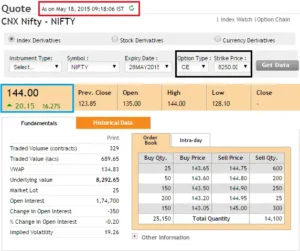
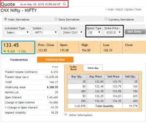
Take note of the following two screenshots, which are from Nifty’s 8250 CE option. The first photo was obtained at 09:18 a.m., when the Nifty was trading at 8292.

A little while later…

Notice the difference in premium – at 09:18 AM, when the Nifty was at 8292, the call option was trading at 144, but by 10:00 AM, the Nifty had climbed to 8315 and the call option was trading at 150.

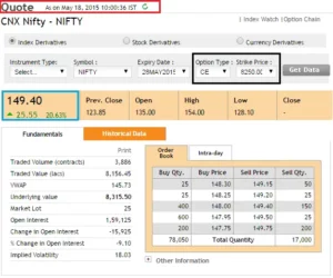
In fact, here’s another image from 10:55 a.m. – The Nifty fell to 8288, as did the option premium (declined to 133).

One thing is evident from the above observations: as the spot price changes so do the option premium. As we already know, the call option premium rises in proportion to the increase in spot value, and vice versa.

Keeping this in mind, imagine you projected that the Nifty will reach 8355 by 3:00 PM today. The images above show that the premium will undoubtedly fluctuate – but by how much? What will the 8250 CE premium be worth if the Nifty reaches 8355?

This is when the ‘Delta of an Option’ comes in helpful. The Delta quantifies how an option’s value moves in relation to the underlying. In simplified terms, an option’s Delta helps us answer queries such as, “How many points would the option premium change for every one point movement in the underlying?”

As a result, Option Greek’s ‘Delta’ measures the effect of market directional movement on the Option’s premium.

The delta is a variable number –

Some traders choose to utilise the 0 to 100 scale for a call option between 0 and 1. So a delta value of 0.55 on a scale of 0 to 1 corresponds to a delta value of 55 on a scale of 0 to 100.
A put option has a value between -1 and 0 (-100 to 0). As a result, a delta value of -0.4 on the -1 to 0 scale corresponds to -40 on the -100 to 0 scale.
We will soon learn why the delta of the put option is negative.
At this point, I’d want to give you an idea of how this chapter will look; please keep this in mind as I believe it will be useful.

At this point, I’d like to give you an idea of how this chapter will look; please keep this in mind as I believe it will help you connect the dots better –

We will learn how to use the Delta value for Call Options.
A simple explanation of how the Delta values are calculated
Learn how to use the Delta value for Put Options.
Delta vs. Spot Characteristics, Delta Acceleration (continued in next chapter)
Delta-based option positions (continued in next chapter)

So let’s get going!

Delta for a Call Option

We know that the delta is a number between 0 and 1. What does it indicate if a call option has a delta of 0.3 or 30?

As we all know, the delta measures the rate of change of the premium for each unit change in the underlying. A delta of 0.3 implies that for every one point change in the underlying, the premium is likely to change by 0.3 units, or for every one hundred point change in the underlying, the premium is likely to change by 30 points.

The following example should help you better grasp this –

Nifty @ 10:55 AM is at 8288

Option Strike = 8250 Call Option

Premium = 133

Delta of the option = + 0.55

Nifty @ 3:15 PM is expected to reach 8310

At 3:15 PM, what is the most likely option premium value?

This is a rather simple calculation. The option’s Delta is 0.55, which means that for every 1-point movement in the underlying, the premium is predicted to vary by 0.55 points.

We estimate the underlying to move by 22 points (8310 – 8288), hence the premium should rise by 22 points.

= 22*0.55

= 12.1

Therefore the new option premium is expected to trade around 145.1 (133+12.1)

Which is the sum of the old premium Plus the predicted premium change?

Consider another scenario: what if one forecasts a decline in the Nifty? What will become of the premium? Let’s sort it out –

Which is the sum of old premium + expected change in premium

Let us pick another case – what if one anticipates a drop in Nifty? What will happen to the premium? Let us figure that out –

Nifty @ 10:55 AM is at 8288

Option Strike = 8250 Call Option

Premium = 133

Delta of the option = 0.55

Nifty @ 3:15 PM is expected to reach 8200

What is the likely premium value at 3:15 PM?

We are expecting Nifty to decline by – 88 points (8200 – 8288), hence the change in premium will be –

= – 88 * 0.55

= – 48.4

Therefore the premium is expected to trade around

= 133 – 48.4

= 84.6 (new premium value)

As shown in the preceding two cases, the delta assists us in determining the premium value depending on the directional movement of the underlying. This knowledge is highly valuable when trading options. Assume you anticipate a tremendous 100-point increase in the Nifty and decide to purchase an option based on this forecast. There are two Call alternatives available, and you must choose one.

Call Option 1 has a delta of 0.05

Call Option 2 has a delta of 0.2

Now the question is, which option will you buy?

Let us do some math to answer this –

Change in underlying = 100 points

Call option 1 Delta = 0.05

Change in premium for call option 1 = 100 * 0.05

= 5

Call option 2 Delta = 0.2

Change in premium for call option 2 = 100 * 0.2

= 20

As you can see, a 100-point move in the underlying has distinct consequences for different possibilities. Clearly, the trader would be better off purchasing Call Option 2. This should give you a hint: the delta assists you in choosing the best option strike to trade. Of course, there are other dimensions to this, which we will investigate shortly.

Let me ask a very critical question at this point: why is the delta value for a call option limited to 0 and 1? Why can’t the delta of a call option go beyond 0 and 1?

To further appreciate this, consider two cases in which I purposefully keep the delta value above 1 and below 0.

Scenario 1: Delta greater than 1 for a call option

Nifty @ 10:55 AM at 8268

Option Strike = 8250 Call Option

Premium = 133

Delta of the option = 1.5 (purposely keeping it above 1)

Nifty @ 3:15 PM is expected to reach 8310

What is the likely premium value at 3:15 PM?

Change in Nifty = 42 points

Therefore the change in premium (considering the delta is 1.5)

= 1.5*42

= 63

Do you see what I mean? According to the answer, a 42-point shift in the underlying increases the value of the premium by 63 points! In other words, the option is increasing in value faster than the underlying. Remember that the option is a derivative contract; its value is derived from the underlying, hence it can never move faster than the underlying.

If the delta is one (the maximum delta value), it indicates that the option is moving in line with the underlying, which is acceptable, but a value greater than one is not. As a result, the delta of an option is limited to a maximum value of 1 or 100.

Scenario 2: Delta lesser than 0 for a call option

Nifty @ 10:55 AM at 8288

Option Strike = 8300 Call Option

Premium = 9

Delta of the option = – 0.2 (have purposely changed the value to below 0, hence negative delta)

Nifty @ 3:15 PM is expected to reach 8200

What is the likely premium value at 3:15 PM?

Change in Nifty = 88 points (8288 -8200)

Therefore the change in premium (considering the delta is -0.2)

= -0.2*88

= -17.6

For a moment we will assume this is true, therefore the new premium will be

= -17.6 + 9

= – 8.6

As you can see in this example, when the delta of a call option falls below zero, the premium also falls below zero, which is impossible. Remember that the premium, whether call or put, can never be negative at this stage. As a result, the delta of a call option is lower limited to zero.

Who decides the value of the Delta?

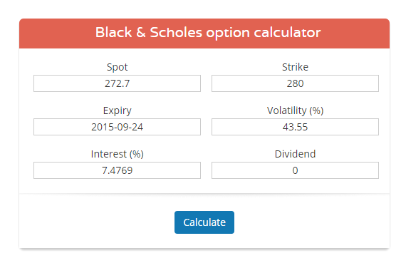
The delta value is one of the numerous outputs of the Black and Scholes option pricing model. As I explained before in this chapter, the B&S formula accepts a large number of inputs and produces a few critical outputs. The option’s delta value and other Greeks are included in the output. After we’ve gone over all of the Greeks, we’ll go through the B&S formula to solidify our comprehension of the alternatives. However, for the time being, you should be aware that the delta and other Greeks are market-driven values determined using the B&S algorithm.

However, the following table will assist you in determining the approximate delta value for a given option –

Option Type	Approx Delta value (CE)	Approx Delta value (PE)
Deep ITM	Between + 0.8 to + 1	Between – 0.8 to – 1
Slightly ITM	Between + 0.6 to + 1	Between – 0.6 to – 1
ATM	Between + 0.45 to + 0.55	Between – 0.45 to – 0.55
Slightly OTM	Between + 0.45 to + 0.3	Between – 0.45 to -0.3
Deep OTM	Between + 0.3 to + 0	Between – 0.3 to – 0

Of course, you may always use a B&S option pricing calculator to determine the exact delta of an option.

Delta for a Put Option

Keep in mind that the Delta of a Put Option might range from -1 to 0. The negative sign simply indicates that when the underlying increases in value, the value of the premium decreases. Consider the following details while keeping this in mind:

Parametres	Value
Underlying	Nifty
Strike	8300
Spot value	8268
Premium	128
Delta	-0.55
Expected Nifty Value (Case 1)	8310
Expected Nifty Value (Case 2)	8230

Note – 8268 is a slightly ITM option, hence the delta is around -0.55 (as indicated from the table above).

The goal is to evaluate the new premium value while keeping the delta value at -0.55. Pay close attention to the calculations below.

Case 1: Nifty is expected to move to 8310

Expected change = 8310 – 8268

= 42

Delta = – 0.55

= -0.55*42

= -23.1

Current Premium = 128

New Premium = 128 -23.1

= 104.9

I’m subtracting the value of delta here because I know that the value of a Put option decreases as the underlying value rises.

Case 2: Nifty is expected to move to 8230

Expected change = 8268 – 8230

= 38

Delta = – 0.55

= -0.55*38

= -20.9

Current Premium = 128

New Premium = 128 + 20.9

= 148.9

I’m including the delta value here since I know that the value of a Put option increases when the underlying value falls.

I hope the following two illustrations have clarified how to use the delta value of the Put Option to calculate the new premium value. Also, I’ll omit describing why the delta of the Put Option is limited to -1 and 0.

In fact, I would encourage readers to utilise the same logic we used to understand why the delta of a call option is bound between 0 and 1 to understand why the delta of a put option is bound between -1 and 0.

In the following chapter, we will delve deeper into Delta and examine some of its properties.

Model Thinking

The preceding chapter provided an overview of the first Greek choice – the Delta. Aside from explaining the delta, the last chapter had another secret agenda: to lead you down the path of’model thinking.’ Let me explain what I mean: the last chapter offered a new window for weighing possibilities. The window opened up several option trading viewpoints; ideally, you no longer think about options in a one-dimensional manner.

For example, if you have a positive market perspective in the future, you may not trade in this manner: ‘My view is optimistic, thus it makes sense to either buy a call option or collect a premium by selling a put option.’

Rather, you may strategy as follows: “My perspective is bullish because I expect the market to move by 40 points; therefore, it makes sense to buy an option with a delta of 0.5 or greater because the option is predicted to gain at least 20 points for the given 40 point move in the market.”

Can you see the distinction between the two cognitive processes? While the former is more naive and casual, the later is more defined and measurable. The expectation of a 20-point increase in the option premium resulted from a calculation discussed in the previous chapter –

Expected change in option premium = Option Delta * Points change in underlying

The given formula is only one part of the whole strategy. As we uncover more Greeks, the evaluation metre gets more quantitative, and trade selection becomes more scientifically streamlined. The point is that future thinking will be directed by formulae and figures, with limited room for “casual trading thoughts.” I know many traders that trade based on a few odd notions, and some of them may be profitable. However, not everyone will enjoy this. When you put numbers in context, your chances improve – and this happens when you develop’model thinking.’

Please keep the model thinking framework in mind when studying options, since this will assist you in setting up systematic trades.

Delta versus the spot price

In the last chapter, we discussed the relevance of Delta and how it may be used to calculate the predicted change in premium. Before we continue, here’s a quick recap of the previous chapter –

The delta of call options is positive. A call option with a delta of 0.4 indicates that for every 1 point increase or decrease in the underlying, the call option premium increases or decreases by 0.4 point.
The delta of put options is negative. A -0.4 delta put option means that for every 1 point loss/gain in the underlying, the put option premium gains/losses 0.4 points.
The delta of TM options is between 0 and 0.5, the delta of ATM options is 0.5, and the delta of ITM options is between 0.5 and 1.

Let me make some deductions based on the third point. Assume the Nifty Spot is at 8312, the strike at issue is 8400, and the option type is CE (Call option, European).

When the spot is 8312, what is the estimated Delta value for the 8400 CE?
Because 8400 CE is OTM, Delta should be between 0 and 0.5. Let us suppose Delta is 0.4.

What do you believe the Delta value is if the Nifty spot moves from 8312 to 8400?
Because the 8400 CE is now an ATM option, the delta should be roughly 0.5.
What do you believe the Delta value is if the Nifty spot moves from 8400 to 8500?
Delta should be closer to one now that the 8400 CE is an ITM option. Let’s pretend it’s 0.8.
Finally, if the Nifty Spot falls sharply from 8500 to 8300, what happens to the delta?
With the drop in spot, the option has reverted to ITM from OTM, and so the delta value has dropped from 0.8 to, say, 0.35.
What conclusions may you draw from the above four points?
Clearly, as and when the spot value changes, so does the moneyness of an option, and therefore the delta.

This is an important element to note: the delta changes as the spot value changes. As a result, delta is a variable rather than a fixed item. As a result, if an option has a delta of 0.4, its value is likely to change in tandem with the underlying’s value.

Take a look at the chart below, which depicts the fluctuation of delta relative to the spot price. The chart is broad and does not pertain to any specific option or strike. There are two lines, as you can see –

The blue line depicts the delta behaviour of the Call option (varies from 0 to 1)
The red line depicts the delta behaviour of the Put option (varies from -1 to 0)

Let us understand this better –

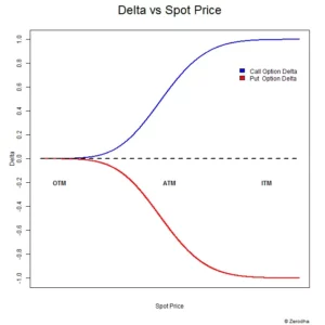
This is an intriguing graphic, and I recommend that you focus just on the blue line and disregard the red line. The delta of a call option is represented by the blue line. The graph above captures a few important delta characteristics; let me list them for you (meanwhile, keep in mind that as the spot price changes, so does the moneyness of the option) –

Examine the X-axis: when the spot price moves from OTM to ATM to ITM, the moneyness increases from left to right.
Examine the delta line (blue line) – as the spot price rises, so does the delta.
At OTM, the delta is flattish near 0 – this means that no matter how much the spot price falls (from OTM to deep OTM), the option’s delta will remain at 0.
Remember that the delta of the call option is lower bound by 0.
When the spot moves from OTM to ATM, the delta begins to rise (remember, the option’s moneyness rises as well).
Take note of how the delta of an option falls between 0 and 0.5 for options less than ATM.
At ATM, the delta reaches 0.5.
When the spot transfers from ATM to ITM, the delta begins to exceed the 0.5 mark.
When the delta reaches a value of one, it begins to plump up.
This also means that once the delta increases beyond ITM, to say deep ITM, the delta value remains constant. It remains at its highest value of one.

The delta of the Put Option exhibits similar features (red line).

The Delta Acceleration

If you are familiar with the options market, you may have heard weird stories about traders doubling or tripling their money by trading OTM options. Let me tell you a story if you haven’t heard one before: The election results were revealed on May 17, 2009 (Sunday), the UPA Government was re-elected at the centre, and Dr.Manmohan Singh was re-elected as the country’s Prime Minister for a second term. Stock markets prefer stability in the centre, and we all anticipated the market would rally the next day, May 18, 2009. The previous day, the Nifty closed at 3671.

Zerodha did not exist at the time; we were simply a group of traders trading our own capital alongside a few clients. One of our associates took a tremendous risk a few days before the 17th of May when he purchased long-term options (OTM) for Rs.200,000/-. Given that no one can truly anticipate the outcome of a general election, this was a daring gesture. Obviously, he would benefit if the market rose, but the market rose for a variety of reasons. We were just as curious as he was to see what would happen. Finally, the results were announced, and we all knew he’d make money on May 18th – but none of us knew how much he’d benefit.

The 18th of May 2009 is a day I will never forget: markets opened at 9:55 a.m. (that was the market opening time back then), it was a big bang open the market, Nifty quickly touched an upper circuit, and the markets froze. Within a few minutes, the Nifty rose nearly 20% to conclude the day at 4321! Because the market was hot, the exchanges decided to close it at 10:01 AM… As a result, I had the shortest working day of my life.

Here is a chart highlighting that day’s market movement –

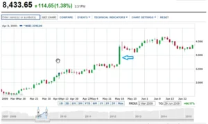
Our good associate had made a lovely fortune throughout the entire process. His option was valued at Rs.28,00,000/- at 10:01 AM on that lovely Monday morning, a staggering 1300 percent gain gained overnight! This is the type of deal that practically all traders, including myself, hope to have.

Anyway, let me ask you a few questions about this story, which will get us back to the primary point –

Why do you believe our employee chose to purchase OTM options rather than ATM or ITM options?
What would have occurred if he had instead purchased an ITM or ATM option?

The answers to these questions can be found in this graph –

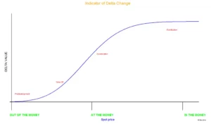
This graph discusses ‘Delta Acceleration’; there are four delta stages indicated in the graph; let us look at each one.

Before we proceed with the following conversation, please consider the following points:

I would recommend that you pay close attention to the following conversation; these are some of the most crucial aspects to understand and remember.
Remember and revise the delta table from the previous chapter (option type, approximate delta value, and so on).
Please keep in mind that the delta and premium amounts used here are an educated guess for the sake of example –

Predevelopment – This is the period where the choice is between OTM and deep OTM. The delta is close to zero in this case. Even if the option moves from deep OTM to OTM, the delta will remain close to zero. For example, if the spot price is 8400, the 8700 Call Option is Deep OTM, with a delta of 0.05. Even if the spot rises from 8400 to, say, 8500, the delta of the 8700 Call option will not change significantly because the 8700 CE is still an OTM option. The delta will remain a tiny non-zero value.

So, if the premium on 8700 CE is Rs.12 when spot is at 8400, the premium is anticipated to move by 100 * 0.05 = 5 points when Nifty moves to 8500 (100 point move).

As a result, the new premium is Rs.12 + 5 = Rs.17/-. The 8700 CE, on the other hand, is now regarded somewhat OTM rather than deeply OTM.

Most importantly, while the rise in premium value is tiny (Rs.5/-), the Rs.12/- option has increased by 41.6 percent to Rs.17/- in percentage terms.

Conclusion – Deep OTM options tend to put on an outstanding percentage, but for this to happen, the spot must move by a significant amount.

Recommendation: Avoid buying deep OTM options because the deltas are extremely small and the underlying must move dramatically for the option to be profitable. There are better values elsewhere. However, selling deep OTM makes sense for the same reason, but we shall examine when to sell these options when we take up the Greek ‘Theta’.

Takeoff and Acceleration – This is the point at which the option changes from OTM to ATM. This is where you get the most bang for your money, and thus the most risk.

Consider the following: Nifty spot at 8400, strike at 8500 CE, option slightly out of the money, delta at 0.25, premium at Rs.20/-

The spot increases from 8400 to 8500 (100 points), therefore let’s do some math to figure out what occurs on the premium side –

underlying change = 100

8500 CE delta = 0.25

Change in premium = 100 * 0.25 = 25

New premium equals Rs.20 + Rs.25 = Rs.45/-

125 percent change in percentage

Do you see what I mean? OTM options respond substantially differently for the same 100 point move.

Conclusion: The somewhat OTM option, with a delta of 0.2 or 0.3, is more sensitive to changes in the underlying. The percentage change in the marginally OTM options is really astounding for any major change in the underlying. In reality, this is exactly how option traders double or triple their money, by purchasing slightly out-of-the-money options when the underlying is expected to move significantly. But I’d like to point out that this is only one face of the cube; there are many more to discover.

Recommendation – Purchasing somewhat OTM options is more expensive than purchasing deep OTM options, but if you play your cards well, you may make a fortune. Consider purchasing slightly OTM options whenever you buy options (of course assuming there is plenty of time to expiry, we will talk about this later).

Let us now look at how the ATM option would react to the same 100-point shift.

Spot = 8400

Strike = 8400 (ATM)

Premium = Rs.60/-

Change in underlying = 100

Delta for 8400 CE = 0.5

Premium change = 100 * 0.5 = 50

New premium = Rs.60 + 50 = Rs.110/-

Percentage change = 83%

Conclusion – ATM options are more susceptible to spot changes than OTM options. Because the ATM’s delta is substantial, the underlying does not need to change by a large amount. Even if the underlying changes only slightly, the option premium changes. However, purchasing ATM options is more expensive than purchasing OTM options.

Recommendation: Purchase ATM options when you want to be safe. Even if the underlying does not move significantly, the ATM option will move. As a corollary, unless you are quite certain of what you are doing, do not attempt to sell an ATM option.

Stabilization – As the option moves from ATM to ITM and Deep ITM, the delta begins to stabilise at one. The delta begins to flatten out as it reaches the value of one, as seen by the graph. This indicates that the option can be ITM or deep ITM, but the delta is set at 1 and does not alter.

Let’s see how this goes.

Nifty Spot = 8400

Option 1 = 8300 CE Strike, ITM option, Delta of 0.8, and Premium is Rs.105

Option 2 = 8200 CE Strike, Deep ITM Option, Delta of 1.0, and Premium is Rs.210

Change in underlying = 100 points, hence Nifty moves to 8500.

Given this let us see how the two options behave –

Change in premium for Option 1 = 100 * 0.8 = 80

New Premium for Option 1 = Rs.105 + 80 = Rs.185/-

Percentage Change = 80/105 = 76.19%

Change in premium for Option 2 = 100 * 1 = 100

New Premium for Option 2 = Rs.210 + 100 = Rs.310/-

Percentage Change = 100/210 = 47.6%

Conclusion – The deep ITM option outperforms the somewhat ITM option in terms of absolute change in the number of points. However, in terms of percentage change, the situation is reversed. Obviously, ITM options are more sensitive to changes in the underlying, but they are also the most expensive.

Most notably, notice the change in the deep ITM option (delta 1) for every 100-point change in the underlying, there is a 100-point change in the option premium. This means that purchasing a deep ITM option is equivalent to purchasing the underlying itself. This is due to the fact that whatever changes occur in the underlying, the deep ITM option will also change.

Recommendation: Purchase the ITM choices if you want to play it safe. When I say safe, I’m referring to the deep ITM choice versus the deep OTM option. ITM options have a high delta, indicating that they are most sensitive to changes in the underlying.

Because a deep ITM option moves in lockstep with the underlying, it can be used to replace a futures contract!

Think about this –

Nifty Spot @ 8400

Nifty Futures = 8409

Strike = 8000 (deep ITM)

Premium = 450

Delta = 1.0

Change in spot = 30 points

New Spot value = 8430

Change in Futures = 8409 + 30 = 8439 à Reflects the entire 30 point change

Change Option Premium = 1*30 = 30

New Option Premium = 30 + 450 = 480 à Reflects the entire 30 point change

So, both futures and Deep ITM options react similarly to changes in the underlying. As a result, you are better off purchasing a Deep ITM option to reduce your margin burden. However, if you choose to do so, you must always ensure that the Deep ITM option remains Deep ITM (in other words, that the delta is always 1), as well as keep an eye on the contract’s liquidity.

I imagine that the knowledge in this chapter is an overdose at this point, especially if you are researching the Greeks for the first time. I recommend that you take your time and learn this one bit at a time.

There are a few more perspectives to investigate about the delta, but we shall do so in the following chapter. However, before we finish this chapter, let us summarise the material using a table.

This table will assist us to understand how different options behave differently when the underlying changes.

I considered Bajaj Auto as the foundation. The price is 2210, and the underlying is expected to change by 30 points (which means we are expecting Bajaj Auto to hit 2240). We’ll also assume there’s plenty of time before expiration, so time isn’t really an issue.

Moneyness	Strike	Delta	Old Premium	Change in Premium	New Premium	% Change
Deep OTM	2400	0.05	Rs.3/-	30* 0.05 = 1.5	3+1.5 = 4.5	50%
Slightly OTM	2275	0.3	Rs.7/-	30*0.3 = 9	7 +9 = 16	129%
ATM	2210	0.5	Rs.12/-	30*0.5 = 15	12+15 = 27	125%
Slightly ITM	2200	0.7	Rs.22/-	30*0.7 = 21	22+21 = 43	95.45%
Deep ITM	2150	1	Rs.75/-	30*1 = 30	75 + 30 =105	40%

As you can see, each option behaves differently for the same underlying move.

Before I finish this chapter, I told you a narrative earlier in this chapter and then asked you a few questions. Perhaps you can go back over the questions again now that you have the answers.

Add up the Deltas

Here’s an intriguing feature of the Delta: the Deltas can be totaled up!

Let me clarify by returning to the Futures contract for a second. We know that for every point movement in the underlying’s spot price, the futures price moves by one point. For instance, if the Nifty Spot goes from 8340 to 8350, the Nifty Futures will move from 8347 to 8357. (i.e. assuming Nifty Futures is trading at 8347 when the spot is at 8340). If we were to apply a delta value to futures, we would plainly assign a delta of one because we know that for every one point change in the underlying, the futures also move by one point.

Assuming I purchase one ATM option with a delta of 0.5, we know that for every one point move in the underlying, the option moves by 0.5 points. In other words, possessing one ATM option is equivalent to holding half a futures contract. Given this, holding two such ATM contracts is equivalent to holding one futures contract because the delta of the two ATM options, 0.5 and 0.5, adds up to a total delta of one! In other words, the deltas of two or more option contracts can be summed to determine the position’s total delta.

Let us look at a few example cases to better grasp this –

Case 1 – Nifty spot at 8125, trader has 3 different Call option.

Sl No	Contract	Classification	Lots	Delta	Position Delta
1	8000 CE	ITM	1 -Buy	0.7	TRUE
2	8120 CE	ATM	1 -Buy	0.5	TRUE
3	8300 CE	Deep OTM	1- Buy	0.05	TRUE
Total Delta of positions					TRUE

Observations –

The ‘Long’ position is indicated by the positive sign next to 1 in the Position Delta column.
The sum of the locations is positive, i.e. +1.25. This suggests that the underlying and combined positions are both moving in the same direction.
The combined position varies by 1.25 points for every one point movement in the Nifty.
If the Nifty moves 50 points, the combined position will move 50 * 1.25 = 62.5 points.

Case 2 – Nifty spot at 8125, trader has a combination of both Call and Put options.

Sl No	Contract	Classification	Lots	Delta	Position Delta
1	8000 CE	ITM	1- Buy	0.7	TRUE
2	8300 PE	Deep ITM	1- Buy	– 1.0	TRUE
3	8120 CE	ATM	1- Buy	0.5	TRUE
4	8300 CE	Deep OTM	1- Buy	0.05	TRUE
Total Delta of positions					0.7 – 1.0 + 0.5 + 0.05 = + 0.25

Observations –

The delta of the combined locations is positive, i.e. +0.25. This suggests that the underlying and combined positions are both moving in the same direction.
With the addition of Deep ITM PE, the overall position delta has decreased, implying that the combined position is less vulnerable to market directional movement.
The combined position varies by 0.25 points for every one point movement in the Nifty.
If the Nifty moves 50 points, the combined position will move 50 * 0.25 = 12.5 points.
It is important to remember that deltas of calls and puts can be added as long as they belong to the same underlying.

Case 3 –Nifty spot at 8125, the trader has a combination of both Call and Put options. He has 2 lots Put option here.

Sl No	Contract	Classification	Lots	Delta	Position Delta
1	8000 CE	ITM	1- Buy	0.7	TRUE
2	8300 PE	Deep ITM	2- Buy	-1	TRUE
3	8120 CE	ATM	1- Buy	0.5	TRUE
4	8300 CE	Deep OTM	1- Buy	0.05	TRUE
Total Delta of positions					0.7 – 2 + 0.5 + 0.05 = – 0.75

Observations –

The delta of the combined positions is negative. This implies that the underlying and combined option positions move in opposite directions.
With the addition of two Deep ITM PE, the entire position has turned delta negative, indicating that the combined position is vulnerable to market direction.
The combined position varies by – 0.75 points for every 1-point movement in the Nifty.
If the Nifty moves 50 points, the position will move 50 * (-0.75) = -37.5 points.

Case 4 – Nifty spot at 8125, the trader has Calls and Puts of the same strike, same underlying.

Sl No	Contract	Classification	Lots	Delta	Position Delta
1	8100 CE	ATM	1- Buy	0.5	TRUE
2	8100 PE	ATM	1- Buy	-0.5	TRUE
Total Delta of positions					+ 0.5 – 0.5 = 0

Observations –

The positive delta of the 8100 CE (ATM) is + 0.5.
The negative delta of the 8100 PE (ATM) is -0.5.
The combined position has a delta of zero, indicating that any change in the underlying position has no effect on the combined position.
For example, if the Nifty moves 100 points, the change in option positions is 100 * 0 = 0.
Positions with a combined delta of 0 are often known as ‘Delta Neutral’ positions.
Any directional shift has no effect on Delta Neutral locations. They act as if they are immune to market fluctuations.
Delta neutral positions, on the other hand, respond to other variables such as volatility and time. This will be discussed at a later time.

Case 5 – Nifty spot at 8125, trader has sold a Call Option

The’short’ position is indicated by the negative sign next to 1 in the Position Delta column.
As we can see, a short call option generates a negative delta, indicating that the option position and the underlying move in opposing directions. This makes sense given that an increase in spot value results in a loss for the call option. seller
Similarly, if you short a PUT option, the delta becomes positive.
-1 * (-0.5) = +0.5

Finally, examine the following scenario: the trader owns a 5 lot long deep ITM option. We know that the total delta for such a position is + 5 * + 1 = + 5. This indicates that for every one point movement in the underlying, the combined position changes by five points in the same direction.

It should be noted that the identical result may be obtained by shorting 5 deep ITM PUT options –

– 5 * – 1 = + 5

-5 represents 5 short positions and -1 represents the delta of deep ITM Put options.

The preceding case study talks should have given you an idea of how to add up the deltas of the individual locations and calculate the overall delta of the positions. When you have many option positions running concurrently and want to detect the overall directional impact on the positions, this technique of adding up the deltas comes in handy.

In fact, I would strongly advise you to always add the deltas of different positions to obtain a perspective – doing so will help you appreciate the sensitivity and leverage of your whole position.

Also, here is another important point you need to remember –

Delta of ATM option = 0.5

If you have 2 ATM options = delta of the position is 1

As a result, for every point change in the underlying, the entire position changes by one point (as the delta is 1). This means that the option’s movement is similar to that of a Futures contract. However, keep in mind that these two options should not be used as a substitute for a futures contract. Remember that the futures contract is solely affected by market direction, whereas options contracts are affected by numerous other variables outside market direction.

There may be instances when you would like to use options instead of futures (mostly for margin purposes), but you must be fully informed of the repercussions of doing so; more on this later.

Max pain & PCR ratio

September 27, 2022August 3, 2022 by Rohansharma

Max pain & PCR ratio

Basics of stock market

• Induction
• Bull call spread
• Bull put spread
• Call ration Back spread
• Bear call ladder
• Synthetic long & Arbitrage
• Bear put spread

• Bear call spread
• put ration back spread
• Long straddle
• Short straddle
• Max pain & PCR ratio
• Iron condor

13.1 – My experience with Option Pain theory

The “Options Pain” theory undoubtedly has a place on the never-ending list of controversial market theories. Option Pain, also known as “Max Pain,” has a sizable fan base, in addition, to probably an equal number of detractors. I’ll be open; I’ve participated on both sides. When I first started investing with Option Pain, I was never able to consistently generate income. Over time, though, I discovered ways to improvise on this theory to fit my own risk tolerance, and that produced a respectable outcome. I’ll go over this as well later in the chapter.

Anyway, this is my attempt to explain the Option Pain theory to you and to discuss my likes and dislikes of Max Pain. This chapter can serve as a guide for how to decide which camp you want to be in.

You must be familiar with the idea of “Open Interest” in order to understand Option Pain theory.

So let’s get going.

13.2 – Max Pain Theory

Here is a step-by-step explanation of how to determine the Max Pain value. You might find this a little perplexing at this point, but I still advise reading it. Things will become more clear once we use an example.

Step 1: Make a list of the different exchange strikes and note the open interest in calls and puts for each strike.

Step 2: Assume that the market will expire at each of the strike prices you have noted.

Step 3: Assuming the market expires as per the assumption in step 2, figure out how much money is lost by option writers (both call option and put option writers).

Step 4: Total the money that calls and put option writers have lost.

Step 5: Determine the strike at which option writers lose the least amount of money.

The point at which option buyers experience the most suffering is the level at which option writers lose the least amount of money. The market will therefore most likely end at this price.

Let’s use a very straightforward example to illustrate this. I’ll assume there are only 3 Nifty strikes available in the market for the purposes of this example. I have noted the open interest for the respective strike for both call and put options.

Situation 1: Assume that the market closes at 7700

Keep in mind that you will only lose money when writing a call option if the market rises above the strike. Similarly, you will only lose money when the market moves below the strike price when you write a put option.

Therefore, none of the call option writers will experience a loss if the market expires at 7700. Therefore, the premiums received by call option writers for the 7700, 7800, and 7900 strikes will be kept.

The writers of put options, however, will have difficulties. The 7900 PE writers will be discussed first.

7900 PE writers would lose 200 points at the 7700 expiries. OI being 2559375, the loss in rupees would be equal to –

= 200 * 2559375 = Rs.5,11,875,000/-

7800 PE writers would suffer a 100 loss.

= 100 * 4864125 = Rs.4,864,125,000/-

It won’t cost 7700 PE writers any money.

Therefore, if the markets expire at 7700, the total amount of money lost by option writers would be –

Call option writers’ total losses plus put option writers’ total losses

= 0 + Rs.511875000 + 4,864125000 = Rs.9,98,287,500/-

Remember that the total amount of money lost by call option writers equals the sum of the losses suffered by writers of 7700 CE, 7800 CE, and 7900 CE.

Similarly, the total amount of money lost by put option writers is equal to the sum of the losses of the writers of the 7700 PE, the 7800 PE, and the 7900 PE.

Scenario 2: Assume that the market closes at 7800.

The writers of the following call options would lose money at 7800:

Using its Open, 7700 CE writers would lose 100 points.

get the loss’s rupee value.

100*1823400 = Rs.1,82,340,000/-

Sellers of the 7800 CE and 7900 CE would both make money.

The seller of the 7700 and 7800 PE wouldn’t suffer a loss.

The loss in rupees would be equal to 100 points for the 7900 PE, multiplied by the open interest.

100*2559375 = Rs.2,55,937,500/-

Therefore, when the market expires at 7800, the total loss for option writers would be –

= 182340000 + 255937500

= Rs.4,38,277,500/-

Scenario 3 – Assume markets expire at 7900

At 7900, the following call option writers would lose money –

7700 CE writer would lose 200 points, the Rupee value of this loss would be –

200 *1823400 = Rs.3,646,800,000/-

7800 CE writer would lose 100 points, and the Rupee value of this loss would be –

100*3448575 = Rs.3,44,857,500/-

7900 CE writers would retain the premiums received.

Since market expires at 7900, all the put option writers would retain the premiums received.

So therefore the combined loss of option writers would be –

= 3646800000 + 344857500 = Rs. 7,095,375,000/-

So at this stage, we have calculated the total Rupee value loss for option writers at every possible expiry level. Let me tabulate the same for you –

get the loss’s rupee value.

100*1823400 = Rs.1,82,340,000/-

We can quickly determine the point at which the market is likely to expire now that we have determined the combined loss that option writers would sustain at various expiry levels.

According to the theory of option pain, the market will expire at a point where option sellers will experience the least amount of suffering (or loss).

The combined loss at this point (7800), which is significantly less than the combined loss at 7700 and 7900, is approximately 43.82 Crores, as can be seen from the table above.

That is all there is to the calculation. For the sake of simplicity, I’ve only used 3 strikes in the example.

For all the available strikes, we assume the market would expire at that point and then compute the Rupee value of the loss for CE and PE option writers. This value is shown in the last column titled “Total Value”. Once you calculate the total value, you simply have to identify the point at which the least amount of money is lost by the option writer. You can identify this by plotting the ‘bar graph’ of the total value. The bar graph would look like this –

As you can see, the 7800 strike is where option writers would lose the least money, so in accordance with the theory of option pain, this is the strike where the market for the May series is most likely to expire.

How can you put this information to use now that you’ve determined the expiry level? Well, there are many applications for this knowledge.

The majority of traders identify the strikes they can write using this maximum pain level. Since 7800 is the anticipated expiration level in this scenario, one can choose to write call options above 7800 or put options below 7800 and keep all of the premiums.

As a result, I eventually modified the traditional option pain theory to fit my risk tolerance. What I did was as follows:

Every day, the OI values change. As a result, the option pain may suggest 8000 as the expiry level on May 20 and 7800 as the expiry level on May 10. To perform this calculation, I froze on a specific day of the month. When there were 15 days left until expiration, I preferred to do this.

In accordance with the standard option pain method, I determined the expiry value.
I would include a “safety buffer” of 5%. The theory suggests 7800 as the expiry at 15 days, so I would then add a 5 percent safety buffer. As a result, the expiration value would be 7800 plus 5% of 7800.

The market could end anywhere between 7800 and 8200, in my opinion.
I would create strategies with this expiration range in mind, with writing call options beyond 8200 being my favourite.
Simply put,

I wouldn’t write a put option because panic spreads more quickly than greed. This implies that markets may decline before rising.

I would typically refrain from averaging during this time and instead hold the sold options until they expired.

13.5 – The Put Call Ratio

Calculating the Put Call Ratio is a fairly straightforward process. The ratio enables us to determine whether the market is extremely bullish or bearish. The PCR test is typically used as a contrarian indicator. In other words, if the PCR shows extreme bearishness, we expect the market to turn around, so the trader adopts a bullish stance. Likewise, traders anticipate a market reversal and decline if the PCR shows extreme bullishness.

Simply dividing the total open interest of Puts by the total open interest of Calls yields the PCR formula. The outcome typically ranges in and around one. Look at the illustration below:

As of 10^th May, the total OI of both Calls and Puts has been calculated. Dividing the Put OI by Call OI gives us the PCR ratio –

37016925 / 42874200 =

0.863385

The following interpretation is correct:

If the PCR value is higher than 1, say 1.3, it means that more puts than calls are being purchased. This indicates that the markets have become very bearish and are thus somewhat oversold. Search for reversals and anticipate an increase in the markets.

Low PCR values, such as 0.5 and below, show that more calls than puts are being purchased. This indicates that the markets have become very bullish and are thus somewhat overbought. One can watch for reversals and anticipate a decline in the markets.
It is possible to attribute all values between 0.5 and 1 to normal trading activity, so they can all be disregarded.

This is obviously a general approach to PCR. It would be sensible to identify these extreme values by historically plotting the daily PCR values over, say, a period of one or two years. For instance, a value of 1.3 for the Nifty can signify extreme bearishness, whereas 1.2 for the Infy could mean the same thing. You must understand this, so backtesting is helpful.

Why PCR is used as a contrarian indicator may be a mystery to you. The reason for this is a little difficult to understand, but the general consensus is that if traders are bullish or bearish, then the majority of them have already taken their respective positions (hence a high/low PCR), and there aren’t many other players who can enter and move the positions in the desired direction. Therefore, when the position eventually squares off, the stock or index will move in the opposite direction.

That’s PCR for you, then. There are numerous variations of this that you may encounter. Some prefer to take volumes instead of OI, while others prefer to take the total traded value. But I don’t believe that overanalyzing PCR is necessary.

13.6 – Final thoughts

And with that, I’d like to conclude the 36 chapters and two modules long module on options!

In this module, we have covered nearly 15 different option strategies, which, in my opinion, is more than enough for retail traders to engage in profitable options trading. Yes, you will come across many fancy option strategies in the future; perhaps your friend will suggest one and demonstrate its technicalities but keep in mind that fancy does not necessarily equate to profitable. The best tactics can sometimes be straightforward, elegant, and straightforward to use.

The information we’ve provided in Modules 5 and 6 are written with the goal of providing you with a clear understanding of what options trading is.

What can be accomplished with options trading and what cannot? What is necessary and what is not have both been considered and discussed. Since these two modules cover the majority of your questions and concerns about options, they are more than enough.

So kindly read through the information provided here at your own pace, and I’m confident you’ll soon begin trading options the right way.

Last but not least, I sincerely hope you enjoy reading this as much as I did writing it for you.

Good luck and keep making money!

For Visit: Click here to know the Directions.

How to buy call option

October 4, 2022August 3, 2022 by Bala gumber

Options

• Option contract
• The option greeks
• Delta
• Gamma
• Theta
• All volatility
• Vega

3.1 – Buying call option

In the preceding chapters, we examined the call option’s fundamental construction and learned the general circumstances in which buying a call option makes sense. We will formally organize our ideas about the call option in this chapter and have a solid understanding of both the purchasing and selling of the call option. Here is a quick summary of everything we learned in the first chapter before continuing with this one:

When you anticipate that the underlying price will rise, it makes sense to purchase a call option.
The buyer of the call option loses money if the underlying price declines or remains unchanged.
The premium (agreement fees) that the buyer pays to the seller/writer of the call option is equal to the amount of money that the buyer of the call option would lose.

We shall keep the aforementioned three considerations in mind (which act as fundamental principles) and gain a deeper understanding of the call option.

3.2 – Building a case for a call option

The purchase of a call option is in a variety of market circumstances. Here is one that I just learned about as I was writing this chapter and thought would be a good fit for our conversations.

Bajaj Auto Limited’s stock is being . They are one of India’s largest two-wheeler manufacturers, as you may know. The stock has been severely undervalued in the market for a number of reasons and is currently trading at its 52-week low. I think there might be a chance to start a trade here. I have the following opinions about this trade:

There is no disputing that Bajaj Auto is a stock with strong fundamentals.
Because of how much the stock has fallen, I think the market may have overreacted to the business cycle instability of Bajaj Auto.
I anticipate that the stock price will finally cease declining and stop short.
But because I’m concerned that the stock will continue to decrease, I don’t want to purchase the stock for delivery (yet).
Extending the previous point, I am unable to purchase Bajaj Auto’s futures due to my concern for M2M losses.
At the same time, I don’t want to pass up a chance for a significant stock price reversal.

In conclusion, I have high hopes for the stock price of Bajaj Auto (which I believe will rise eventually), but I have some trepidation regarding the stock’s near-term prospects. The major source of uncertainty is the potential severity of my short-term losses in the event that the stock’s decline continues. However, based on my estimation, the likelihood of the loss is minimal, but it is still possible. So what do I need to do?

As you can see, I’m in a situation that Ajay was in at the same time (recall the Ajay – Venu example from chapter 1). This kind of situation sets up a classic example of an options transaction.

In light of my predicament, purchasing a call option on Bajaj Auto makes sense for the reasons I’ll discuss in a moment.

As shown, the stock is currently trading at Rs. 2026.9. (highlighted in blue). With a premium of Rs. 6.35, I’ll decide to purchase a call option with a strike price of 2050. (highlighted in the red box and red arrow). You might be wondering why, since there are so many other strike prices available (highlighted in green), I chose the 2050 strike price. We will ultimately cover the process of choosing a strike price in this module, but for now, let’s assume that 2050 is the appropriate strike price to trade.

3.3 – Intrinsic value of a call option (upon expiry)

What transpires with the call option now that the expiration is 15 days away? In general, there are three possibilities that could occur, which I assume you are already aware of:

The stock price rises above the strike price, say 2080, in scenario one.

Scenario 2: The stock price declines to 2030, which is below the strike price.

The stock price remains at 2050 in scenario three.

I’ll also presume that you are familiar with the P&L calculation at the precise value of the spot in the three scenarios above as they are fairly similar to the ones we looked at in chapter 1. (if not, I would suggest you read through Chapter 1 again).

The concept I’m presently interested in investigating is this:

You will concur that there are just three major categories in which the price movement of Bajaj Auto may be (following expiration), namely, the price either rises, falls, or remains unchanged.
What about all the other prices in between, though? For instance, in Scenario 1, the price is set at 2080, which is higher than the striking price of 2050. What about further strike prices like 2055, 2060, 2065, 2070, etc.? Can we draw any conclusions about the P&L from this?
In scenario 2, the price is anticipated to be around 2030, which is less than the 2050 strike. How about more strike prices like 2045, 2040, 2035, etc.? Having said that, anything here with respect to the P&L?

I would want to refer to these points as the “Conceivable values of the spot on expiry” in order to generalize the P&L knowledge of the call option. What would happen to the P&L at various possible spot prices (upon expiry)?

To start, I’d like to discuss the concept of the “intrinsic value of the option at expiry” (in part, not the complete concept).

The non-negative value that the option buyer would be to if he were to exercise the call option is known as the intrinsic value (IV) of the option upon expiration (particularly a call option for now). Simply put, determine how much cash you would receive at expiration if the call option you own were profitable (assuming you are the buyer of the call option). It is in mathematics as –

IV = Strike Price – Spot Price

Therefore, the 2050 Call option’s intrinsic value would be if Bajaj Auto is trading at 2068 on the day of expiration (in the spot market).

= 2068 – 2050

= 18

Likewise, the intrinsic value of the option would be – if Bajaj Auto is trading at 2025 on the expiry day.

= 2025 – 2050

= -25

But keep in mind that the IV of an option is always a positive figure, whether it is a call or a put.

= 0

Now, our goal is to keep the notion of the option’s intrinsic worth in perspective, determine how much money I will make at each potential Bajaj Auto expiration value, and use that information to draw some broad conclusions about the P&L of call option buyers.

3.4 – Generalizing the P&L for a call option buyer

Now that we’ve kept the idea of an option’s intrinsic value in the back of our minds, let’s work to create a table that will show us how much money I, as the buyer of Bajaj Auto’s 2050 call option, would earn under the various potential spot value changes of Bajaj Auto (in the spot market) on expiration. Keep in mind that Rs 6.35 was as the premium for this choice. The fact that I Rs.6.35 remains intact, regardless of how the spot value fluctuates. This is the expense I incurred to purchase the 2050 Call Option.

What then do you notice? The table above reveals two notable observations:

The most that might be, even if Bajaj Auto’s price drops (below the strike price of 2050), appears to be just Rs. 6.35/-

1. Generalization 1: When the spot price declines below the strike price, the buyer of a call option suffers a loss. However, the call option buyer’s loss is only as great as the premium he has .

2. When Bajaj Auto begins to rise over the 2050 strike price, the profit from this call option appears to grow rapidly.

Generalization 2: When the spot price rises above the strike price, the call option is lucrative. The profit increases as the difference between the strike price and the current price rises.

3. The buyer of the call option has a restricted risk and the potential to earn a limitless profit, according to the aforementioned two generalizations.

The Call option P&L for a specific spot price can be using the following generic formula:

Max [0, (Spot Price – Strike Price)] = P&L – Premium

Let’s examine the P&L for a few potential spot values on expiry using the formula above:

2023 \s2072 \s2055

The answer is as follows:

@2023

= Max [0, (2023 – 2050)] – 6.35

= Max [0, (-27)] – 6.35

= 0 – 6.35

= – 6.35

The resolution fits Generalization 1 (loss restricted to the extent of the premium ).

@2072

= Max [0, (2072 – 2050)] – 6.35

= Max [0, (+22)] – 6.35

= 22 – 6.35

= +15.65

The solution fits Generalization 2. (Call option gets profitable as and when the spot price moves over and above the strike price).

@2055

= Max [0, (2055 – 2050)] – 6.35

= Max [0, (+5)] – 6.35

= 5 – 6.35

= -1.35

This presents a challenging circumstance because the outcome goes against the second generalization. The trade is losing money even though the spot price is higher than the strike price! What causes this? Furthermore, the actual loss is substantially lower than the maximum loss of Rs. 6.35/-; it is just Rs. 1.35/-. We need carefully examine the P&L activity surrounding the spot value, which is marginally over the strike price, to ascertain why this is occurring (2050 in this case).

As you can see from the table above, until the spot price reaches the strike price, the buyer incurs a maximum loss (in this example, Rs. 6.35). The loss begins to diminish, though, once the spot price begins to rise above the strike price. Up until a moment where neither a profit nor a loss is from the trade, the losses are continuously. The breakeven point is what we refer to as.

Any call option’s breakeven point can be using the following formula:

B.E. = Strike Price Plus Premium

The “Break Even” point for the Bajaj Auto example is –

= 2050 + 6.35

= 2056.35

Let’s actually determine the P&L at the breakeven point.

= Max [0, (2056.35 – 2050)] – 6.35

= Max [0, (+6.35)] – 6.35

= +6.35 – 6.35

= 0

As you can see, at the breakeven point, we are in the negative financially. In other words, for the call option to become profitable, it must move above both the strike price and the breakeven point.

3.5 – Call option buyer’s payoff

We have already discussed a few crucial aspects of a call option buyer’s payment, so let me restate them here:

The greatest loss a call option buyer can incur is equal to the premium amount. As long as the spot price is lower than the strike price, the buyer loses money.
If the current price rises over the strike price, the buyer of the call option could benefit indefinitely.
Even though the call option is meant to provide income when the spot price rises above the strike price, the buyer must first recoup the premium he has already paid.
The breakeven point is the point at which the buyer of a call option fully recoups the premium he has paid.
Only after passing the breakeven mark does the call option buyer actually begin to benefit (which naturally is above the strike price)

The following points, which are consistent with our recent discussion, can be seen in the graphic above:

As long as the spot price is trading at any price below the strike of 2050, the loss is limited to Rs. 6.35.
Losses can be shown to decrease from 2050 to 2056.35 (breakeven price).
We can see that there is no profit or loss at 2056.35.
The call option starts to profit above 2056.35. In reality, the P&L line’s slope plainly shows that when the spot value moves away from the strike, the profits begin to rise exponentially.

One thing is clear from the graph once more: A call option buyer has low risk but unlimited profit potential. And with that, I hope you have a better understanding of the call option from the standpoint of the buyer. We shall examine the Call Option from the seller’s standpoint in the following chapter.

CONCLUSION

When you anticipate that the underlying price will rise, it makes sense to purchase a call option.
The buyer of the call option loses money if the underlying price declines or remains unchanged.
The premium (agreement fees) that the buyer pays to the seller/writer of the call option is equal to the amount of money that the buyer of the call option would lose.
A call option’s intrinsic value (IV) is a non-negative number.
IV = Max[0, strike price minus spot price]
The maximum loss a call option buyer can incur is equal to the premium they paid. As long as the spot price is lower than the strike price, a loss is incurred.
If the current price rises over the strike price, the buyer of the call option could benefit indefinitely.
Even though the call option is meant to provide income when the spot price rises above the strike price, the buyer must first recoup the premium he has already paid.
The breakeven point is the point at which the buyer of a call option fully recoups the premium he has paid.
Only after passing the breakeven mark does the call option buyer actually begin to benefit (which naturally is above the strike price).

Short straddle

September 27, 2022August 3, 2022 by Rohansharma

Short straddle

Basics of stock market

• Induction
• Bull call spread
• Bull put spread
• Call ration Back spread
• Bear call ladder
• Synthetic long & Arbitrage
• Bear put spread

• Bear call spread
• put ration back spread
• Long straddle
• Short straddle
• Max pain & PCR ratio
• Iron condor

11.1 – Context

In the previous chapter we understood that for the long straddle to be profitable, we need a set of things to work in our favor, reposting the same for your quick reference –

The volatility should be relatively low at the time of strategy execution
The volatility should increase during the holding period of the strategy
The market should make a large move – the direction of the move does not matter
The expected large move is time bound, should happen quickly – well within the expiry
Long straddles are to be set up around major events, and the outcome of these events is to be drastically different from the general market expectation.

Although it is acknowledged that the long straddle does not depend on the direction of the market, this is a very difficult bargain. Considering the five points listed, it can be difficult to make the long straddle work in your favour. Remember that the breakdown in the previous chapter was at 2%; add another 1% for desired profits, and we are essentially looking for at least a 3% movement on the index. According to my experience, it can be difficult to anticipate the market’s frequent changes. In fact, just for this reason, I pause every single time I need to start a long straddle.

I’ve seen a lot of traders carelessly set up long straddles in the mistaken belief that they are protected from the direction of the market. However, in reality, they lose money in a long straddle because of time delays and the market’s overall movement (or lack thereof). Please note that I’m not trying to convince you not to use the long straddle; nobody contests its simplicity and elegance. When all five of the aforementioned criteria are met, it functions incredibly well. The likelihood of these 5 points aligning with one another is the only problem I have with long straddle.

Consider this: A number of factors prevent the long straddle from being profitable. Therefore, as a continuation of this, the same set of factors “should” favour the “Short Straddle,” which is the opposite of a long straddle.

11.2 – The Short Straddle

Although many traders fear the short straddle (as losses are uncapped), I personally prefer trading the short straddle on certain occasions over its peer strategies. Anyway, let us quickly understand the setup of a short straddle, and how its P&L behaves across various scenarios.

Setting up a short straddle is quite straightforward – as opposed to buying the ATM Call and Put options (like in a long straddle) you just have to sell the ATM Call and Put option. Obviously, the short strategy is set up for a net credit, as when you sell the ATM options, you receive the premium in your account.

Here is an example, consider Nifty is at 7589, so this would make the 7600 strike ATM. The option premiums are as follows –

7600 CE is trading at 77
7600 PE is trading at 88

So the short straddle will require us to sell both these options and collect the net premium of 77 + 88 = 165.

Please keep in mind that the options must have the same underlying, the same expiration date, and of course, the same strike. Let’s calculate the P&L under various market expiry scenarios assuming that you have already executed this short straddle.

Situation 1: The market closes at 7200 (we lose money on the put option)

In this case, the put option’s loss is so sizable that it consumes the premium that both the CE and the PE collected, resulting in a net loss. At 7200 –

As a result of the fact that 7600 CE will expire worthlessly, we keep the premium received, meaning that 77 7600 PE will have an intrinsic value of 400. When the premium received, Rs. 88, is taken into account, we lose 400 – 88 = – 312.
312 – 77 = – 235 would be the overall loss.
As you can see, the loss in the put option equals the gain in the call option.

The market expires at 7435 in scenario two (lower breakdown)

In this instance, the strategy is in a neutral financial position.

Since 7600 CE would expire worthlessly, the premium is kept. Profit is Rs. 77 here.
Since we received Rs. 88 in premium on an intrinsic value of 165 for 7600 PE, our loss would be 165 – 88 = -77.
The loss in the put option completely cancels out the gain in the call option. Consequently, at 7435, we are in the black.

Situation 3: The market closes at 7600 (at the ATM strike, maximum profit)

The best result for a short straddle is this one. The situation is simple at 7600 because both the call and put options would expire worthlessly and the premiums from both the call and put options would be kept. The gain, in this case, would equal the net premium received, or Rs. 165.

This indicates that in a short straddle, you profit the most when the markets remain static.

The market expires at 7765 in scenario 4. (upper breakdown)

This is comparable to the second scenario we looked at. At this point, the strategy achieves parity at a point above the ATM strike.

After accounting for the premium of Rs. 77 that was received, 7600 CE would have an intrinsic value of Rs. 165, meaning that we would lose Rs. 88. (165 – 77)
7600 PE would expire worthlessly, so the premium, which is equal to Rs. 88, is kept.

We are neither making money nor losing money because the profit from the 7600 PE is offset by the loss from the 7600 CE.

This is undoubtedly the upper breakdown point.

In this case, the market is obviously much larger than the 7600 ATM threshold. Both the loss and the call option premium would increase.7600 PE will expire worthlessly, so the premium, which is equal to Rs. 88, is kept.

After accounting for the premium of Rs. 77 received, the 7600 CE will have an intrinsic value of Rs. 400 at 8000, meaning that we will lose Rs. 323. ( 400 -77)
Given that we paid Rs. 88 as the put option premium, our loss would be equal to 88 – 323 = –235.

As you can see, the call option’s loss is sizable enough to cancel out the total premiums paid.

The payoff table for various market expiries is shown below.

11.3 – Case Study (repost from previous module)

He decided to proceed with the 1140 strike because Infosys was trading close to Rs. 1142/- per share (ATM).

Here is the snapshot taken at the time the trade was started:

The 1140 CE was trading at 48/- on October 8 around 10:35 AM, and the implied volatility was 40.26 percent. The implied volatility was 48 percent and the 1140 PE was trading at 47/-. 95 dollars per lot were received in total premium.

The market anticipated that Infosys would release a respectable set of financial results. In fact, the results were better than anticipated; the specifics are as follows:

“Information Systems reported a net profit of $519 million for the July-September quarter, up from $511 million in the same period last year. The amount of revenue increased by 8.7% to $2.39 billion. Revenue increased by 6% sequentially, comfortably exceeding market expectations of growth of 4- 4.5%.

On revenues of Rs. 15,635 crores, which was up 17.2 percent from the previous year, net profit increased by 9.8 percent to Rs. 3398 crores in rupees. Economic Times is the source.

Three minutes after the market opened and around the time of the announcement, at 9:18 AM, this trader was able to close the trade.

5.4 – Effect of Greeks

Since we are dealing with ATM options, the delta of both CE and PE would be around 0.5. We could add the deltas of each option and get a sense of how the overall position deltas behave.

Given that we are short, the delta for the 7600 CE would be -0.5.
Since we are short, the delta for the 7600 PE Delta would be +0.5.
Delta added together would be -0.5 + 0.5 = 0.
The total delta shows that the tactic is neutral in terms of direction. Keep in mind that a delta-neutral straddle can be either long or short. Delta neutral suggests that the profits are uncapped for long straddles and the losses are uncapped for short straddles.

Here’s something to consider: When you start a straddle, you are undoubtedly delta neutral. But will your position still be delta neutral as the markets change? If so, why do you believe that? If the answer is no, is there a way to maintain a neutral position delta?

I can assure you that your understanding of options is far superior to that of 90% of market participants if you can structure your thinking around these ideas. You must take a small mental step forward and enter second-level thinking in order to respond to these straightforward questions.

For Visit: Click here to know the directions.

Options

21.1 – Background

21.2 – Overview of the model

21.3 – Put Call Parity

Options

5.1 – Getting the orientation right

5.2 – Building a case for a Put Option buyer

5.3 – Intrinsic Value (IV) of a Put Option

5.4 – P&L behavior of the Put Option buyer

5.5 – Put option buyer’s P&L payoff

CONCLUSION

Options

7.1 – Remember these graphs

7.2 – Option Buyer in a nutshell

7.2 – Option seller in a nutshell

Options

6.1 – Building the case

6.2 – P&L behavior for the put option seller

6.3 – Put option seller’s Payoff

Options

4.1 – Two sides of the same coin

4.2 – Call option seller and his thought process

4.3 – Call Option seller pay-off

4.4 – A note on margins

4.5 – Putting things together

4.6 – European versus American Options

CONCLUSION

Basics of stock market

14.1 – New margin framework

We are living in fascinating times, especially if you trade options in India.

The NSE’s new margin framework, which goes into effect on June 1, 2020, reduces the margin requirement for the hedged position.

You might wonder what a hedged position is. Although we have already covered this topic extensively in this module, we will quickly go over it again to ensure that this chapter is comprehensive.

This means that whenever you start a hedged strategy, your broker will block fewer margins than would be needed for a naked position.

In the new margin framework, NSE essentially made the same suggestion.

For more information, see this NSE presentation.

The presentation is quite complex, but unless you really want to, you won’t need to scratch your head to understand it.

There are three main lessons to be learned from the new margin policy from the perspective of a trader. All three are highlighted on a single slide in this presentation. Here is a quick summary:

Starting from the top –

Portfolio 1 – Margins have increased for naked unhedged positions to 18.5% from the current 16.7%.

Portfolio 2 – 70% reduction in margins for market-neutral positions

Portfolio 3 – 80% reduction in margins for spread positions

What does this mean for you as a trader of options?

So some of the practical strategies that on paper looked great but were impossible to implement due to excessive margin requirements, now appear alluring.

I have a trick question for you: Why do you believe the spread position’s margin reduction is greater than that of a neutral market position?

Please consider it and share your thoughts in the comment section.

Given this, I would like to talk about one more options strategy in this module. Previously, I had refrained from doing so because the margin requirement was so high, but that is no longer the case.

14.2 – Iron Condor

An alternative setup with four legs is the iron condor. An improvement on the short strangle is the iron condor.

Check out this –

This screenshot was taken using Sensibull’s Strategy Builder. As you can see, I’m attempting to set up a short strangle by selling OTM calls and puts while Nifty is at 9972.9.

9800 Put at 165.25 10100 Dial 145.25.

The fact that both options are written/sold entitles me to the sum of 164.25 + 145.25 = 309.5 in premium.

I would advise you to read this chapter if you are unfamiliar with the strangles.

This short strangle setup has the following payoff:

Since you sell or write options in a short strangle, you receive a net premium credit. You receive a premium of Rs. 23,288 in this situation.

The exposed ends of short strangles are the only drawback. If the underlying asset changes direction, the strategy bleeds.

For instance, the safety range for this specific short strangle is between 9490 and 10411.

I concur that this is a wide enough range, but markets have shown us that they are capable of making absurd moves very quickly. The most recent crash was COVID-19 in early 2020, which was quickly recovered from.

If you are caught in a market move that is moving so quickly, the potential loss could be enormous and could empty your account. The risk to you and the broker is now quite high because the amount of loss that could occur is limitless. Eventually, this also results in higher margins.

5.3 – Strategy Generalization

which is quite expensive.

This does not, however, mean that you must abandon a quick strangle. The short strangle can be modified to create an iron condor, which is a much better tactic in my opinion.

By closing the ends, an iron condor improvises a short strangle. Consider an iron condor in three sections:

Part 1: Sell a slightly OTM Call and Put option to set up a short strangle.

Part 2: Purchase an additional OTM Call to hedge the short call against a significant market rally.

Part 3: Purchase an additional OTM Put to hedge the short Put against a large market.

An iron condor is a four-legged option strategy as a result. Let’s see how this appears.

Sell a 10100CE at 145.25 and a 9800PE at 165.25 to earn a premium of 310.5 or Rs. 23,288.

Buy 10300 CE at 77 to cover the short position on 10100 CE in part two.

Buy 9600 PE at 105.05 to cover the short 9800 PE in part three.

If you give this some thought, you can see that the long option positions are funded by the short option premium.

Because you purchase two options to hedge against two short options, the profit potential is somewhat diminished –

As you can see, the maximum profit is now Rs. 9,634; however, the decreased profit also results in less stress.

Because I can now see the risk and it isn’t open-ended, the maximum loss is now limited to Rs. 5,366, which in my opinion is awesome.

As long as Nifty stays within a range—in this case, between 9672 and 10228—the profit is constrained. In comparison to the short strangle, observe how the range has decreased.

The iron condor’s payoff is as follows:

Now, what do you think about the risk? The risk here is completely defined. You have clear visibility of the worst-case scenario. So what does it mean to you as a trader, and what does it mean to the broker?

You guessed it right since the risk is defined, the margins are lesser.

Here is where the NSE’s new margin framework is put to use. When compared to the short strangle, which has a margin requirement of Rs. 1.45L, an iron condor only requires you to pay an upfront margin of Rs. 44,303.

Additionally, executing an iron condor was not a very viable option for a retail trader prior to the new margin framework. The margin needed for an Iron Condor was roughly between 2 and 2.2L for these strikes and premiums.