Options

• Basics of call options
• Basics of options jargon
• How to buy a call option
• How to buy/sell call option
• Buying put option
• Selling put option
• Call & put options
• Greeks & calculator

• Option contract
• The option greeks
• Delta
• Gamma
• Theta
• All volatility
• Vega

How many of you recall doing mathematics in high school? Do the terms differentiation and integration sound familiar? Back then, the term “derivatives” meant something else to all of us: it simply referred to solving long differentiation and integration problems.

Let me try to refresh your memory – the goal here is to simply get a point through without delving into the complexities of solving a calculus issue. Please keep in mind that the next topic is very significant to possibilities; please continue reading.

Consider the following:

A car gets started and travels for 10 minutes till it reaches the third-kilometer point. The car goes for another 5 minutes from the 3rd-kilometer point to the 7th-kilometer mark.

Let us focus and note what really happens between the 3^rd and 7^th kilometer, –

Let ‘x’ = distance, and ‘dx’ the change in distance
Change in distance i.e. ‘dx’, is 4 (7 – 3)
Let ‘t’ = time, and ‘dt’ the change in time
Change in time i.e. ‘dt’, is 5 (15 – 10)

If we divide dx over dt i.e. change in distance over change in time we get ‘Velocity’ (V)!

V = dx / dt

= 4/5

This means the car travels 4 kilometres every 5 minutes. The velocity is expressed in kilometres per minute here, which is clearly not a convention we use in everyday language because we are used to expressing speed or velocity in kilometres per hour (KMPH).

By performing a simple mathematical change, we can convert 4/5 to KMPH –

When stated in hours, 5 minutes = 5/60 hours; inserting this into the preceding equation

= 4 / (5/ 60)

= (4*60)/5

= 48 Kmph

Hence the car is moving at a velocity of 48 kmph (kilometers per hour).

Remember that velocity is defined as the change in distance travelled divided by the change in time. In the field of mathematics, speed or velocity is known as the ‘first order derivative’ of distance travelled.

Let us expand on this example: the car arrived at the 7th Kilometer after 15 minutes on the first leg of the voyage. Assume that in the second leg of the voyage, beginning at the 7th-kilometer mark, the car continues for another 5 minutes and arrives at the 15th-kilometer mark.

We know the car’s velocity on the first leg was 48 kmph, and we can easily compute the velocity on the second leg as 96 kmph (dx = 8 and dt = 5).

The car clearly travelled twice as fast on the second portion of the excursion.

Let us refer to the change in velocity as ‘dv.’ Change in velocity is also known as ‘Acceleration.’

We know that the velocity change is

= 96KMPH – 48 KMPH

= 48 KMPH /??

The above response implies that the velocity change is 48 KMPH…. but over what? Isn’t it perplexing?

Allow me to explain:

** The following explanation may appear to be a digression from the main topic of Gamma, but it is not, so please continue reading; if nothing else, it will refresh your high school physics **

When you go to buy a new car, the first thing the salesman tells you is, “the car is incredibly quick since it can accelerate from 0 to 60 in 5 seconds.” Essentially, he is stating that the car can accelerate from 0 KMPH (total rest) to 60 KMPH in 5 seconds. The velocity change here is 60KMPH (60 – 0) in 5 seconds.

Similarly, in the above case, we know the difference in velocity is 48KMPH, but over what distance? We won’t know what the acceleration is unless we answer the “over what” question.

We can make several assumptions to determine the acceleration in this particular scenario –

Constant acceleration
For the time being, we can disregard the 7th-kilometer mark and focus on the fact that the car was at the 3rd-kilometer mark at the 10th minute and reached the 15th-kilometer mark at the 20th minute.

Using the preceding information, we can deduce further information (known as the ‘starting conditions’ in calculus).

Velocity @ the 10th minute (or 3rd kilometer mark) = 0 KMPS. This is called the initial velocity
Time lapsed @ the 3rd kilometer mark = 10 minutes
Acceleration is constant between the 3rd and 15th kilometer mark
Time at 15th kilometer mark = 20 minutes
Velocity @ 20th minute (or 15th kilometer marks) is called ‘Final Velocity”
While we know the initial velocity was 0 kmph, we do not know the final velocity
Total distance travelled = 15 – 3 = 12 kms
Total driving time = 20 -10 = 10 minutes
Average speed (velocity) = 12/10 = 1.2 kmps per minute or in terms of hours it would be 72 kmph

Now think about this, we know –

Initial velocity = 0 kmph
Average velocity = 72 kmph
Final velocity =??

By reverse engineering we know the final velocity should be 144 Kmph as the average of 0 and 144 is 72.

Further we know acceleration is calculated as = Final Velocity / time (provided acceleration is constant).

Hence the acceleration is –

= 144 kmph / 10 minutes

10 minutes, when converted to hours, is (10/60) hours, plugging this back into the above equation

= 144 kmph / (10/60) hour

= 864 Kilometers per hour.

This means the car is gaining 864 kilometres per hour, and if a salesman were to sell you this car, he would state it can accelerate from 0 to 72kmph in 5 seconds (I’ll let you do the arithmetic).

We greatly simplified this problem by assuming that acceleration is constant. In fact, however, acceleration is not constant; you accelerate at varied rates for obvious reasons. To calculate such problems involving changes in one variable as a result of changes in another variable, one must first learn derivative calculus, and then apply the notion of ‘differential equations.

Just consider this for a bit –

Change in distance travelled (position) = Velocity, often known as the first order derivative of distance position.

Acceleration = Change in Velocity

Acceleration is defined as a change in velocity over time, which results in a change in position over time.

As a result, it is appropriate to refer to Acceleration as the 2nd order derivative of position or the 1st derivative of Velocity!

Keep this fact about the first and second-order derivatives in mind as we move on to understanding the Gamma.

Drawing Parallels

We learned about Delta of choice in the previous chapters. As we all know, delta reflects the change in premium for a given change in underlying price.

For example, if the Nifty spot price is 8000, we know the 8200 CE option is out-of-the-money, so its delta might be between 0 and 0.5. For the sake of this conversation, let’s set it to 0.2.

Assume the Nifty spot rises 300 points in a single day, which means the 8200 CE is no longer an OTM option, but rather a slightly ITM option. As a result of this increase in spot value, the delta of the 8200 CE will no longer be 0.2, but rather somewhere between 0.5 and 1.0.

One thing is certain with this shift in underlying: the delta itself changes. Delta is a variable whose value varies according to changes in the underlying and premium! Delta is extremely similar to velocity in that its value changes as time and distance are changed.

An option’s Gamma estimates the change in delta for a given change in the underlying. In other words, the Gamma of an option helps us answer the question, “What will be the equivalent change in the delta of the option for a given change in the underlying?”

let us assume 0.8.

Let us now reintroduce the velocity and acceleration example and draw some connections to Delta and Gamma.

1^st order Derivative

The change in distance travelled (position) with respect to time is recorded by velocity, which is known as the first order derivative of position.

Delta captures the change in premium with regard to the change in underlying, and so delta is known as the premium’s first order derivative.

2^nd order Derivative

Acceleration captures the change in velocity with respect to time, and acceleration is known as the 2nd order derivative of position.
Gamma captures changes in delta with respect to changes in the underlying value; thus, Gamma is known as the premium’s second order derivative.

As you might expect, calculating the values of Delta and Gamma (and any other Option Greeks) requires a lot of number crunching and calculus (differential equations and stochastic calculus).

Here’s a fun fact for you: derivatives are so-called because the value of the derivative contract is determined by the value of the underlying.

This value that derivative contracts derive from their respective basis is assessed through the use of “Derivatives” as a mathematical notion, which is why Futures and Options are referred to as “Derivatives.”

You might be interested to hear that there is a parallel trading universe where traders use derivative calculus to locate trading opportunities on a daily basis. Such traders are known as ‘Quants’ in the trading world, which is a somewhat sophisticated term. Quantitative trading is what resides on the other side of the ‘Markets’ mountain.

Understanding the 2nd order derivative, such as Gamma, is not an easy process in my experience, however, we will try to simplify it as much as possible in the next chapters.

The Curvature

We now know that the Delta of an option is a variable because its value changes in response to changes in the underlying. Let me repost the delta movement graph here –

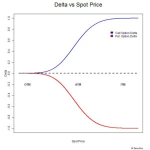
Looking at the blue line showing the delta of a call option, it is evident that it travels between 0 and 1, or possibly from 1 to 0, depending on the situation. Similar observations may be made on the red line indicating the delta of the put option (except the value changes from 0 to 1). This graph underlines what we already know: the delta is a variable that changes over time. Given this, the question that must be answered is –

I’m aware of the delta changes, but why should I care?
If the delta change is important, how can I estimate the likely delta change?

We’ll start with the second question since I’m very positive the answer to the first will become clear as we proceed through this chapter.

As discussed in the previous chapter, ‘The Gamma’ (2nd order derivative of premium), also known when the option’s curvature, is the rate at which the option’s delta varies as the underlying changes. The gamma is typically stated in deltas gained or lost per one-point change in the underlying, with the delta increasing by the gamma when the underlying rises and falling by the gamma when the underlying falls.

For example, consider this –

Nifty Spot = 8326
Strike = 8400
Option type = CE
Moneyness of Option = Slightly OTM
Premium = Rs.26/-
Delta = 0.3
Gamma = 0.0025
Change in Spot = 70 points
New Spot price = 8326 + 70 = 8396
New Premium =??
New Delta =??
New moneyness =??

Let’s figure this out –

Change in Premium = Delta * change in spot i.e 0.3 * 70 = 21
New premium = 21 + 26 = 47
Rate of change of delta = 0.0025 units for every 1 point change in underlying
Change in delta = Gamma * Change in underlying i.e 0.0025*70 = 0.175
New Delta = Old Delta + Change in Delta i.e 0.3 + 0.175 = 0.475
New Moneyness = ATM

When the Nifty moved from 8326 to 8396, the 8400 CE premium increased from Rs.26 to Rs.47, and the Delta increased from 0.3 to 0.475.

The option switches from slightly OTM to ATM with a shift of 70 points. That indicates the delta of the choice must change from 0.3 to close to 0.5. This is exactly what is going on here.

Let us also imagine that the Nifty rises another 70 points from 8396; let us see what occurs with the 8400 CE option –

Old spot = 8396
New spot value = 8396 + 70 = 8466
Old Premium = 47
Old Delta = 0.475
Change in Premium = 0.475 * 70 = 33.25
New Premium = 47 + 33.25 = 80.25
New moneyness = ITM (hence delta should be higher than 0.5)
Change in delta =0.0025 * 70 = 0.175
New Delta = 0.475 + 0.175 = 0.65

Let’s take this forward a little further, now assume Nifty falls by 50 points, let us see what happens with the 8400 CE option –

Old spot = 8466
New spot value = 8466 – 50 = 8416
Old Premium = 80.25
Old Delta = 0.65
Change in Premium = 0.65 *(50) = – 32.5
New Premium = 80.25 – 32. 5 = 47.75
New moneyness = slightly ITM (hence delta should be higher than 0.5)
Change in delta = 0.0025 * (50) = – 0.125
New Delta = 0.65 – 0.125 = 0.525

Take note of how smoothly the delta transitions and follows the delta value principles we learned in previous chapters. You may also be wondering why the Gamma value is kept constant in the preceding samples. In reality, the Gamma also changes as the underlying changes. This change in Gamma caused by changes in the underlying is recorded by the 3rd derivative of the underlying, which is known as “Speed” or “Gamma of Gamma” or “DgammaDspot.” For all practical reasons, it is unnecessary to discuss Speed unless you are mathematically inclined or work for an Investment Bank where the trading book risk can be in the millions of dollars.

In contrast to the delta, the Gamma is always positive for both Call and Put options. When a trader is long options (both calls and puts), he is referred to as a ‘Long Gamma,’ and when he is short options (both calls and puts), he is referred to as a ‘Short Gamma.’

Consider this: the Gamma of an ATM Put option is 0.004, what do you believe the new delta is if the underlying moves 10 points?

Before you proceed, I would like you to take a few moments to consider the above solution.

The solution is as follows: Because we are discussing an ATM Put option, the Delta must be approximately -0.5. Remember that put options have a negative delta. As you can see, gamma is a positive number, i.e. +0.004. Because the underlying moves by 10 points without stating the direction, let us investigate what happens in both circumstances.

Case 1 – Underlying moves up by 10 points

Delta = – 0.5
Gamma = 0.004
Change in underlying = 10 points
Change in Delta = Gamma * Change in underlying = 0.004 * 10 = 0.04
New Delta = We know the Put option loses delta when underlying increases, hence – 0.5 + 0.04 = – 0.46

Case 2 – Underlying goes down by 10 points

Delta = – 0.5
Gamma = 0.004
Change in underlying = – 10 points
Change in Delta = Gamma * Change in underlying = 0.004 * – 10 = – 0.04
New Delta = We know the Put option gains delta when underlying goes down, hence – 0.5 + (-0.04) = – 0.54

Here’s a trick question for you: We’ve already established that the Delta of a Futures contract is always 1, therefore what do you believe the gamma of a Futures contract is? Please share your responses in the comment section below:).

Estimating Risk using Gamma

I know that many traders set risk limitations while trading. Here’s an illustration of what I mean by a risk limit: suppose a trader has Rs.300,000/- in his trading account. Each Nifty Futures contract requires a margin of roughly Rs.16,500/-. Please keep in mind that you can utilise Zerodha’s SPAN calculator to determine the margin necessary for any F&O contract. So, taking into account the margin and the M2M margin necessary, the trader may decide at any point that he does not want to hold more than 5 Nifty Futures contracts, thereby establishing his risk limitations; this seems reasonable and works well when trading futures.

Does the same rationale apply when trading options? Let’s see if this is the correct way to think about risk when trading options.

Consider the following scenario:

Lot size = 10 lots traded (Note: 10 lots of ATM contracts with 0.5 delta each equals 5 Futures contracts.)

Number of lots traded = 10 lots (Note – 10 lots of ATM contracts with a delta of 0.5 each is equivalent to 5 Futures contracts)
Option = 8400 CE
Spot = 8405
Delta = 0.5
Gamma = 0.005
Position = Short

The trader is short 10 lots of Nifty 8400 Call Option, indicating that he is trading within his risk tolerance. Remember how we talked about adding up the delta in the Delta chapter? To calculate the overall delta of the position, we can simply add up the deltas. Furthermore, each delta of one indicates one lot of the underlying. So we’ll keep this in mind and calculate the delta of the overall position.

Delta = 0.5
Number of lots = 10
Position Delta = 10 * 0.5 = 5

So, in terms of overall delta, the trader is within his risk limit of trading no more than 5 Futures lots. Also, because the trader is short options, he is effectively short gamma.

The delta of the position is 5, which means that the trader’s position will move 5 points for every 1 point movement in the underlying.

Assume the Nifty moves 70 points against him and the trader maintains his position, looking for a recovery. The trader clearly believes that he is holding 10 lots of options, which are within his risk tolerance…

Let’s do some forensics to figure out what’s going on behind the scenes –

Delta = 0.5
Gamma = 0.005
Change in underlying = 70 points
Change in Delta = Gamma * change in underlying = 0.005 * 70 = 0.35
New Delta = 0.5 + 0.35 = 0.85
New Position Delta = 0.85*10 = 8.5

Do you see the issue here? Despite having set a risk limit of 5 lots, the trader has exceeded it due to a high Gamma value and now owns positions worth 8.5 lots, much above his perceived risk limit. An inexperienced trader may be taken off guard by this and continue to believe he is well below his danger threshold. In actuality, his risk exposure is increasing.

Suggest you read that again in small bits if you found it confusing.

But since the trader is short, he is essentially short gamma…this means when the position moves against him (as in the market moves up while he is short) the deltas add up (thanks to gamma) and therefore at every stage of market increase, the delta and gamma gang up against the short option trader, making his position riskier way beyond what the plain eyes can see. Perhaps this is the reason why they say – shorting options carry a huge amount of risk. In fact, you can be more precise and say “shorting options carry the risk of being short gamma”.

Note – By no means I’m suggesting that you should not short options. In fact, a successful trader employs both short and long positions as the situation demands. I’m only suggesting that when you short options, you need to be aware of the Greeks and what they can do to your positions.

Also, I’d strongly suggest you avoid shorting option contracts which has a large Gamma.

This leads us to another interesting topic – what is considered a ‘large gamma’.

Gamma movement

We briefly examined the Gamma changes in relation to the change in the underlying earlier in the chapter. The 3rd order derivative named ‘Speed’ captures this shift in Gamma. For the reasons stated previously, I will refrain from discussing ‘Speed.’ However, we must understand the behaviour of Gamma movement in order to prevent beginning trades with high Gamma. Of course, there are other benefits to understanding Gamma behaviour, which we shall discuss later in this lesson. But for now, we’ll look at how the Gamma reacts to changes in the underlying.

Take a look at the graph below.

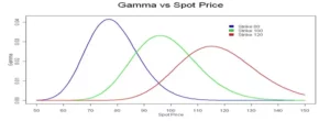
The chart above depicts three alternative CE strike prices – 80, 100, and 120 – as well as their corresponding Gamma movement. The blue line, for example, represents the Gamma of the 80 CE strike price. To minimise misunderstanding, I recommend that you examine each graph separately. In actuality, for the sake of clarity, I will only discuss the 80 CE strike option, which is represented by the blue line.

Assume the spot price is at 80, resulting in the ATM at 80. Keeping this in mind, we can see the following from the preceding chart –

Because the strike under consideration is 80 CE, the option becomes ATM when the spot price equals 80 CE.
Strike values less than 80 (65, 70, 75, etc.) are ITM, while values more than 80 (85, 90, 95, etx) are OTM.
The gamma value for OTM Options is low (80 and above). This explains why the premium for OTM options does not change substantially in absolute point values but changes significantly in percentage terms. For example, the premium of an OTM option can rise from Rs.2 to Rs.2.5, and while the absolute change is only 50 paisa, the percentage change is 25%.
When the option reaches ATM status, the gamma increases. This suggests that the rate of change of delta is greatest when ATM is selected. In other words, ATM options are particularly vulnerable to changes in the underlying.
Also, avoid shorting ATM options because they have the biggest Gamma.
The gamma value for ITM options is also low (80 and below). As a result, for a given change in the underlying, the rate of change of delta for an ITM option is substantially lower than for an ATM option. However, keep in mind that the ITM option has a significant delta by definition. As a result, while ITM delta reacts slowly to changes in the underlying (because to low gamma), the change in premium is significant (due to high base value of delta).
Other strikes, such as 100 and 120, exhibit similar Gamma behaviour. In fact, the purpose of displaying different strikes is to demonstrate how the gamma operates consistently across all options strikes.

If the preceding talk was too much for you, here are three basic points to remember:

For the ATM option, the delta varies quickly.
Delta for OTM and ITM options changes slowly.
Never sell ATM or ITM options in the belief that they would expire worthless.
OTM options are excellent candidates for short trades if you intend to retain them until expiry and expect the option to expire worthless.

Quick note on Greek interactions

Understanding how individual option Greeks perform under different conditions is one of the keys to effective options trading. Now, in addition to knowing individual Greek behaviour, one must also comprehend how these individual option Greeks interact with one another.

So far, we have just analysed the premium change in relation to changes in the current price. We haven’t talked about time or volatility yet. Consider the markets and the real-time changes that occur. Time, volatility, and the underlying pricing all change. As a result, an options trader should be able to grasp these changes and their overall impact on the option premium.

This will only be completely appreciated if you grasp how the option Greeks interact with one another. Typical Greek cross interactions are gamma versus time, gamma versus volatility, volatility versus time, time versus delta, and so on.

Finally, all of your knowledge about the Greeks comes down to a few key decision-making elements, such as –

Which strike is the best to trade under the current market conditions?
What do you think the premium for that particular strike will be – will it rise or fall? As a result, would you be a buyer or a seller in that scenario?
Is there a reasonable chance that the premium may rise if you buy an option?
Is it safe to short an option if you intend to do so? Are you able to detect danger beyond what the naked eye can see?

All of these questions will be answered if you thoroughly grasp individual Greeks and their interactions.

Given this, here is how this module will evolve in the future –

So far, we’ve figured out Delta and Gamma.
We shall learn about Theta and Vega in the next chapters.
When we present Vega (change in premium due to change in volatility), we will take a brief detour to comprehend volatility-based stoploss.
Introduce Greek cross interactions such as Gamma vs Time, Gamma versus Spot, Theta versus Vega, Vega versus Spot, and so on.
An explanation of the Black and Scholes option pricing formula
Calculator of options

So, as you can see, we have a long way to go before we sleep:-).

Conclusion

The rate of change of delta is measured by gamma.
For both Calls and Puts, Gamma is always a positive value.
Large Gamma can be associated with high risk (directional risk)
You are long Gamma when you buy options (calls or puts).
When you sell options (calls or puts), you sell Gamma.
Avoid shorting options with a high gamma.
For the ATM option, the delta varies quickly.
Delta for OTM and ITM options changes slowly.

To know more about the Stock Market Courses Call Rajouri Garden 8595071711 or Noida 8920210950

Gamma